1. 概述
在本篇文章中,我们将讲解如何高效地找出两个已排序数组中的公共元素。这个问题在算法和实际开发中都非常常见,比如在合并数据、查找交集等场景中都有应用。
2. 问题描述
我们有两个升序数组:
a = [a₁ ≤ a₂ ≤ … ≤ aₙ]b = [b₁ ≤ b₂ ≤ … ≤ bₘ]
我们的任务是找出这两个数组中所有公共元素,并保证输出结果也是升序排列的。数组中允许有重复元素,结果中也要体现重复的次数。
举个例子:
a = [1, 2, 2, 4, 5]b = [2, 2, 2, 3, 5, 7]
那么输出应该是:[2, 2, 5]
3. 线性时间解法(双指针法)
✅ 思路
既然两个数组都是有序的,我们可以使用双指针法来线性扫描两个数组,逐个比较当前元素:
- 如果
a[i] < b[j],说明a[i]不可能是公共元素,移动i - 如果
a[i] > b[j],同理,移动j - 如果相等,说明找到一个公共元素,加入结果数组,并同时移动
i和j
这种方法类似于归并排序中“合并”两个数组的步骤。
✅ 伪代码
algorithm LinearAlgorithmForCommonElements(a, b):
    c <- an empty array
    i <- 1
    j <- 1

    while i <= n and j <= m:
        if a[i] < b[j]:
            i <- i + 1
        else if b[j] < a[i]:
            j <- j + 1
        else:
            append a[i] to c
            i <- i + 1
            j <- j + 1

    return c
✅ 时间复杂度
- **O(n + m)**:每个数组只被遍历一次,效率非常高
✅ 示例演示(图解)
初始状态:
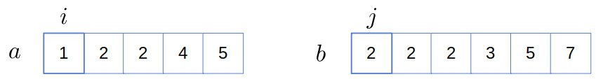
逐步比较:
a[0] = 1 < b[0] = 2→ i++a[1] = 2 == b[0]→ 加入结果,i++, j++a[2] = 2 == b[1]→ 加入结果,i++, j++- ...
- 最终结果:
[2, 2, 5]
4. 对数时间解法(二分查找 + 双指针优化)
⚠️ 适用场景
当其中一个数组远小于另一个时,比如 m << n,我们可以考虑对较小数组中的每个元素,在较大数组中做二分查找。
✅ 优化思路
- 遍历数组
b中的每个元素b[j] - 对
a执行二分查找,判断b[j]是否存在 - 同时利用
a是有序数组的特性进行优化:每次查找后可以将查找起点后移,避免重复搜索前面的元素
✅ 伪代码
algorithm FindCommonElementsBinarySearch(a, b):
    c <- an empty array
    k <- 1
    j <- 1

    while j <= m and k <= n:
        k <- BINARY-SEARCH(b[j], a[k:n])

        if b[j] == a[k]:
            append b[j] to c
            k <- k + 1
        else:
            if j < m and b[j+1] > b[j]:
                k <- k + 1

        j <- j + 1

    return c
✅ 时间复杂度
- 最坏情况:O(m log n)
- 如果
m远小于n,可以近似看作 **O(log n)**,效率非常高 - 如果
m ≈ n,则为 **O(n log n)**,虽然不如线性算法,但比暴力解法好很多
5. 总结对比
| 方法 | 时间复杂度 | 适用场景 | 优点 | 缺点 |
|---|---|---|---|---|
| 暴力解法(双重循环) | O(n * m) | 无排序信息 | 简单直接 | 性能差 |
| 双指针法(线性扫描) | O(n + m) | 两数组都排序 | 高效、简单 | 仅适用于有序数组 |
| 二分查找法 | O(m log n) | 其中一个数组远小于另一个 | 高效 | 实现略复杂,需注意查找起点优化 |
✅ 建议:优先使用双指针法,除非你知道其中一个数组特别小,才考虑使用二分查找法。
💡 踩坑提醒:
- 不要忽略重复元素的处理
- 不要忘记边界条件判断(如指针越界)
- 二分查找时注意起始位置优化,否则可能退化为 O(m log n) 的低效版本
🔚 总结:
两个有序数组找公共元素是一个非常经典的算法问题。使用双指针法可以在 O(n + m) 时间内高效解决,是首选方案。在特定条件下(如小数组查找),二分查找法也能发挥优势。掌握这两种方法,能帮助你在实际开发和算法面试中游刃有余。