鸡尾酒排序

1. Overview

In this tutorial, we’re going to explain what the cocktail sort is and how it works. We’ll also look at the complexity analysis of this sorting algorithm and share the difference between cocktail sort and bubble sort algorithms. What we do is that we actually extend the bubble sort in a way that works in two directions.

2. How Does the Cocktail Sort Work?

Cocktail sort is also known as cocktail shake sort, shaker sort, or bidirectional bubble sort. It is basically an extension of the bubble sort. Like its extension, we use it to teach rather than apply it to real problems. Because, as we guess, its complexity is not different from the bubble sort and it’s not convenient to use in real problems especially with larger inputs.

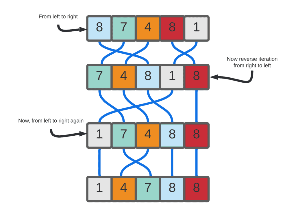
Let’s look at the figure below and understand how it works:

As we’ve seen, we have an array with the size of four for the simplicity of the example. We need to compare each element at index with the element at index+1 while going from left to right. That’s why we’ll end up with the array in the second row of the figure. So, now our iterator points to the last element and we can go back from the end of the array to where it begins instead of starting all over again.

This is where the cocktail name comes from actually. At this iteration, we should compare the element at index with the element at index-1 because we’re going backward, from right to left. After this, we’ll have the array in the third row of the figure. Now our iterator points to the first element again and if we forward again, we’ll end up with a sorted version of our original array. There won’t be any swap operation in this iteration and the cocktail sort will finish its job.

So, as we see, it’s really similar to bubble sort. That’s why it’s called a bi-directional bubble sort as well.

2.1. Pseudocode of the Cocktail Sort

Let’s see the pseudocode of the cocktail sort algorithm:

algorithm CocktailSort(A):
    // INPUT
    //    A = the array to sort
    // OUTPUT
    //    The array A is sorted

    swapped <- true

    while swapped:
        swapped <- false

        for i <- 0 to (length(A) - 2):
            if A[i] > A[i + 1]:
                swap(A[i], A[i + 1])
                swapped <- true

        if not swapped:
            break

        swapped <- false

        for i <- (length(A) - 2) to 0:
            if A[i] > A[i + 1]:
                swap(A[i], A[i + 1])
                swapped <- true

Let’s discuss the algorithm above to get more intuition about cocktail sort. Our goal is to take input array and sort its elements in ascending order.

We have a variable which is a flag that indicates whether we should continue to swap elements in the array or stop doing the sorting.

As we talked about before we have two passes on the given array in cocktail sort. In the first for each loop*,* we’re going from left to right and searching for suitable swap operations. After this loop ends, we’ll end up at the last element of the array.

If there is no swap until this point, we can break the loop. If we swap the elements at least once, now we should go back from the right to the beginning of the array. We’re doing this with the second for each loop*,* this makes us go in the reverse direction. We’re repeating this for each loop until no swap operation occurs.

At the end of the algorithm, we have a sorted version of the array .

3. Complexity Analysis

The time complexity of the cocktail sort in big O notation is on the worst case and the average case. However, if the list is close to ordered before applying the sorting algorithm, its complexity becomes close to .

For instance, there are some cases where each element is at a position that changes at most from the position it will end up at, and the complexity of the cocktail sort will be equal to .

On the other hand, since we know that it’s the variation of the bubble sort algorithm, and the bubble sort algorithm isn’t better than insertion sort, we can infer that it’s not suitable for large inputs. As we mentioned earlier, it’s more suitable for educational purposes like its ancestor.

The space complexity of the cocktail sort algorithm is since it sorts in place.

4. Differences Between the Cocktail Sort and the Bubble Sort

There are slight differences between the cocktail sort and the bubble sort. Cocktail sort passes through the list both from left to right and from right to left. However, bubble sort just passes through in one direction in each iteration.

Another advantage of the cocktail sort is that since it checks the list in both directions, the range of possible swaps will reduce per pass. However, this affects the performance slightly, so it doesn’t even affect the complexity at all.

5. Conclusion

In this article, we’ve shared what the cocktail sort or cocktail shaker sort is, and how it works. We’ve also explained its complexity in terms of time and space. We concluded the article with the difference between the bubble sort and the cocktail sort.