1. 概述
本文将介绍两种常用的查找算法:哈希查找(Hash Lookup) 与 二分查找(Binary Search),并从时间复杂度的角度进行对比分析。
这两种算法在数据结构和实际应用中都非常常见。简单来说:
- 哈希查找:适用于无序数据集合,通过哈希函数快速定位目标数据。
- 二分查找:要求数据集合有序,通过不断缩小查找范围提高效率。
我们最终会从最佳、平均、最坏情况下对两者进行性能对比,帮助你在不同场景下做出合理选择。
2. 哈希查找
2.1 什么是哈希查找?
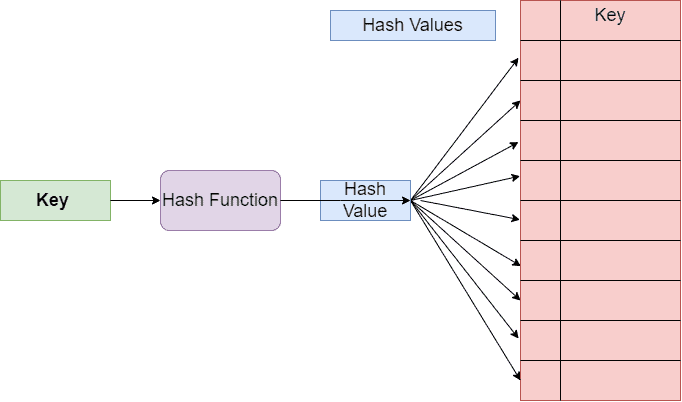
哈希查找基于 哈希表(Hash Table) 实现。哈希表是一种通过键(Key)快速访问值(Value)的数据结构。它通过 哈希函数(Hash Function) 将任意长度的键映射为一个固定长度的索引值(Hash Value),然后将数据存储在该索引位置。
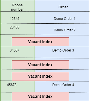
举个例子:一家餐厅要记录外卖订单,用户输入手机号作为查询依据。如果直接用手机号作为索引,会浪费大量空间。因此,餐厅可以使用一个哈希函数将手机号转换为一个较小的数字作为索引。
如下图所示,原始电话号码作为索引占用空间大且容易冲突:
通过哈希函数处理后,索引空间大幅压缩:
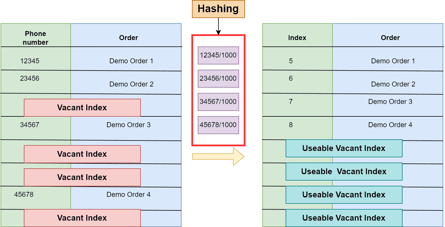
最终形成一个哈希表结构:
2.2 哈希冲突问题
由于哈希函数输出范围有限,多个不同的键可能映射到同一个索引上,这就是 哈希冲突(Collision)。
解决冲突的常见方法有:
- 链地址法(Separate Chaining):每个索引维护一个链表,用于存储多个冲突的键值对。
- 开放地址法(Open Addressing):线性探测、二次探测等方法。
2.3 时间复杂度分析
| 场景 | 时间复杂度 | 说明 |
|---|---|---|
| 最佳情况 | ✅ O(1) | 无冲突,直接命中 |
| 平均情况 | ✅ O(1) | 冲突较少,链表长度均衡 |
| 最坏情况 | ❌ O(n) | 所有键都映射到同一索引,退化为线性查找 |
哈希查找的效率高度依赖于哈希函数的设计和负载因子(Load Factor)。
3. 二分查找
3.1 什么是二分查找?
二分查找是一种基于 有序数组 的查找算法,采用 分治策略(Divide and Conquer),每次将搜索区间缩小一半。
示例流程:
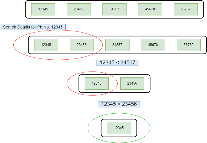
假设我们要查找电话号码 12345,数组已按升序排列:
- 找到中间元素
34567,比目标值大 → 查找左半部分。 - 中间元素为
11111,比目标值小 → 查找右半部分。 - 找到目标值
12345。
如下图所示:
3.2 时间复杂度分析
| 场景 | 时间复杂度 | 说明 |
|---|---|---|
| 最佳情况 | ✅ O(1) | 目标正好是中间元素 |
| 平均情况 | ✅ O(log n) | 每次将查找范围减半 |
| 最坏情况 | ✅ O(log n) | 目标位于最左或最右端 |
⚠️ 注意:二分查找要求输入数组必须是有序的。如果数据频繁变动,需要额外维护排序结构,否则无法使用。
4. 时间复杂度对比总结
| 场景 | 哈希查找 | 二分查找 |
|---|---|---|
| 最佳情况 | ✅ O(1) | ✅ O(1) |
| 平均情况 | ✅ O(1) | ✅ O(log n) |
| 最坏情况 | ❌ O(n) | ✅ O(log n) |
对比分析:
- 在最佳情况下,两者表现相同。
- 在平均情况下,哈希查找更优,适合频繁查找的场景。
- 在最坏情况下,二分查找更稳定,不会因哈希冲突导致性能下降。
使用建议:
| 使用场景 | 推荐算法 |
|---|---|
| 数据无序、需频繁查找 | 哈希查找 |
| 数据有序、查找频率中等 | 二分查找 |
| 数据频繁变动、需排序结构 | 二分查找 |
| 需要稳定最坏时间复杂度 | 二分查找 |
5. 总结
哈希查找和二分查找各有优劣:
- ✅ 哈希查找:速度快、适合无序数据,但最坏情况性能差。
- ✅ 二分查找:稳定、适合有序数据,但不支持无序结构。
在实际开发中,选择哪种方式应根据数据特性、访问频率和性能要求综合判断。比如:
- 如果你维护一个缓存系统,推荐使用 哈希查找。
- 如果你处理的是静态有序数据(如配置表、字典),推荐使用 二分查找。
理解它们的底层原理和适用场景,能让你在性能优化和系统设计中游刃有余。