1. Introduction
While writing any research article or technical documents in LaTeX, we often have to demonstrate an algorithm according to our proposed model, workflow, or architecture.
In this tutorial, we’ll explore three approaches to writing pseudocode in LaTeX. Firstly, we’ll discuss the algorithmic package, followed by the algorithmicx package. Lastly, we’ll discuss the algorithm2e package. Notably, all three packages require the algorithm wrapper.
2. Using the algorithmic Package
The algorithmic package is one of the straightforward ways to write algorithms in LaTeX. Moreover, it offers a simple syntax for describing algorithms, making it suitable for basic algorithmic representations. In addition, it supports basic loop constructs and conditional statements.
Hence, we can use the algorithmic package to write algorithms in LaTeX.
2.1. Example
Now, let’s look at the example of Quicksort algorithm using the algorithmic package:
\documentclass{article}
\usepackage{algorithm}
\usepackage{algorithmic}
\begin{document}
\begin{algorithm}
\caption{Quick Sort}
\begin{algorithmic}[1]
    \STATE \textbf{Procedure} \textsc{QuickSort}($A$, $low$, $high$)
        \IF{$low < high$}
            \STATE $pivotIndex \gets \textsc{Partition}(A, low, high)$
            \STATE \textsc{QuickSort}(A, low, pivotIndex - 1)
            \STATE \textsc{QuickSort}(A, pivotIndex + 1, high)
        \ENDIF
    \STATE \textbf{End Procedure}
\end{algorithmic}
\end{algorithm}
\begin{algorithm}
\caption{Partition}
\begin{algorithmic}[1]
        \STATE \textbf{Procedure} \textsc{Partition}($A$, $low$, $high$)
            \STATE $pivot \gets A[high]$
            \STATE $i \gets low - 1$
            \FOR{$j \gets low$ \textbf{to} $high - 1$}
                \IF{$A[j] \leq pivot$}
                    \STATE $i \gets i + 1$
                    \STATE swap $A[i]$ and $A[j]$
                \ENDIF
            \ENDFOR
            \STATE swap $A[i + 1]$ and $A[high]$
            \RETURN $i + 1$
        \STATE \textbf{End Procedure}
\end{algorithmic}
\end{algorithm}
\end{document}
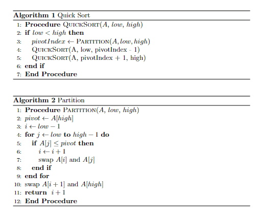
Now, Let’s look at the compiled LaTeX code for the sample document:

Hence, we see two algorithms in the output.
2.2. Explanation
In the above example, we wrap the LaTeX code in the algorithm wrapper. The structure and commands provided by the algorithm and algorithmic packages help in formatting and organizing the algorithm steps clearly.
To elaborate, the algorithm package provides the algorithm environment to wrap the entire algorithm, and the algorithmic package provides the algorithmic environment, which is defined by \begin{algorithmic}[1] and \end{algorithmic}. After that, we set the title of the algorithm using \caption.
Following this, we establish the algorithmic environment defined by \begin{algorithmic}[1] and \end{algorithmic}. Moreover, the [1] argument specifies that every line should be numbered. Subsequently, we use the \STATE \textbf{Procedure} \textsc{QuickSort}($A$, $low$, $high$) command to define a procedure:
- \STATE introduces new steps as well as provides easy referencing of specific steps in the algorithm
- \textbf{Procedure} emphasizes that a procedure is being defined
- \textsc{QuickSort} typesets the procedure name in small caps for emphasis and clarity
- ($A$, $low$, $high$) defines the parameters of the procedure
Furthermore, the algorithmic package also supports commands for conditional statements and iterations, such as \IF and \FOR. Additionally, we use the \RETURN statement to specify the value to be returned by the procedure. Notably, we end each block with its respective end tag, such as \ENDIF and \ENDFOR.
However, the algorithmic package does not support indentation of the algorithm steps, which can make the structure of more complex algorithms harder to follow. This is a limitation to consider when deciding whether to use this package for algorithm representations.
3. The algorithmicx Package
The algorithmicx package is an extension of the well-known algorithmic package. Moreover, it provides a set of macros for creating algorithms in LaTeX documents. Furthermore, its versatility allows users to design algorithms in various styles, including pseudocode, flowcharts, and structured programming constructs.
3.1. Example
Now, let’s write this pseudocode into LaTeX using algorithmicx:
\documentclass{article}
\usepackage{algorithm}
\usepackage{algpseudocode}
\begin{document}
\begin{algorithm}
\caption{Quick Sort}
\begin{algorithmic}[1]
    \Function{QuickSort}{$A, low, high$}
        \If{$low < high$}
            \State $pivotIndex \gets \Call{Partition}{A, low, high}$
            \State \Call{QuickSort}{$A, low, pivotIndex - 1$}
            \State \Call{QuickSort}{$A, pivotIndex + 1, high$}
        \EndIf
    \EndFunction
\end{algorithmic}
\end{algorithm}
\begin{algorithm}
\caption{Partition}
\begin{algorithmic}[1]
    \Function{Partition}{$A, low, high$}
        \State $pivot \gets A[high]$
        \State $i \gets low - 1$
        \For{$j \gets low$ \textbf{to} $high - 1$}
            \If{$A[j] \leq pivot$}
                \State $i \gets i + 1$
                \State Swap $A[i]$ and $A[j]$
            \EndIf
        \EndFor
        \State Swap $A[i + 1]$ and $A[high]$
        \State \Return $i + 1$
    \EndFunction
\end{algorithmic}
\end{algorithm}
\end{document}
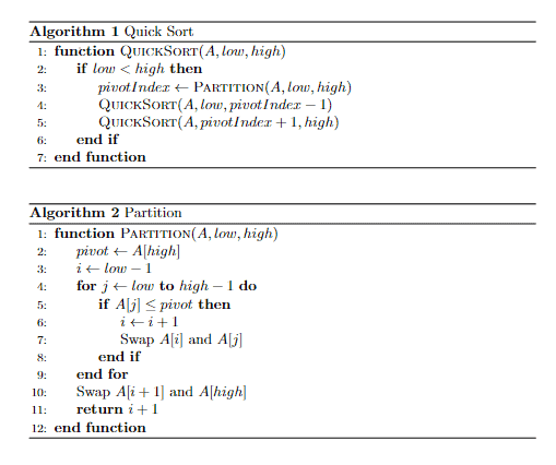
Let’s look at the compiled document:

Here, we can see that the output looks similar to the algorithmic package. However, it provides better indentation of the algorithm.
3.2. Explanation
Let’s break down the provided LaTeX code and see how algorithmicx is different from algorithmic.
In the above code, we import the algpseudocode package, which is part of the algorithmicx bundle and provides the environment and commands for typesetting pseudocode in algorithms.
Within this environment, we define the Quick Sort function using the \Function command. Moving forward, we use \State to introduce a new step in the algorithm. Moreover, this code also uses \Call to call another function in the pseudocode.
In summary, this LaTeX code effectively demonstrates how to present the Quick Sort algorithm using the algpseudocode package. The commands \Function, \If, \For, \State, and \Return help structure the pseudocode clearly, while the line numbering enhances readability and reference.
4. The algorithm2e Package
The algorithm2e package offers more flexibility and customization options compared to algorithmic. Moreover, it provides a more intuitive syntax and supports various formatting choices for algorithms. Additionally, we can use its other formatting and customization options, such as line numbering and indentation settings.
4.1. Example
For the demonstration of the algorithm2e package, we’ll write the Quicksort algorithm:
\documentclass{article}
\usepackage[linesnumbered,ruled,vlined]{algorithm2e}
\begin{document}
\begin{algorithm}
\caption{Quick Sort}
\SetKwFunction{FQuickSort}{QUICKSORT}
\SetKwFunction{FPartition}{PARTITION}
\SetKwProg{Fn}{Function}{:}{}
\Fn{\FQuickSort{$A, low, high$}}{
    \If{$low < high$}{
        $pivotIndex \gets \FPartition(A, low, high)$\;
        \KwCall{\FQuickSort{$A, low, pivotIndex - 1$}}\;
        \KwCall{\FQuickSort{$A, pivotIndex + 1, high$}}\;
    }
}
\Fn{\FPartition{$A, low, high$}}{
    $pivot \gets A[high]$\;
    $i \gets low - 1$\;
    \For{$j \gets low$ \KwTo $high - 1$}{
        \If{$A[j] \leq pivot$}{
            $i \gets i + 1$\;
            Swap $A[i]$ and $A[j]$\;
        }
    }
    Swap $A[i + 1]$ and $A[high]$\;
    \KwRet{$i + 1$}\;
}
\end{algorithm}
\end{document}
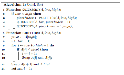
Let’s look at the sample output that we get after compiling the LaTeX document:

From the above output, we can see that the algorithms has created two functions for the Quicksort algorithm.
4.2. Explanation
The provided LaTeX code utilizes the algorithm2e package to write an algorithm. Let’s break down each part.
We utilize the algorithm2e package to present the Quick Sort algorithm. In this code, we initially include the algorithm2e package using the command \usepackage[linesnumbered,ruled,vlined]{algorithm2e}. This statement allows for line numberings, horizontal rules, and vertical lines.
Following this, the code defines two functions: QuickSort and Partition, using \SetKwFunction{FQuickSort}{QuickSort} and \SetKwFunction{FPartition}{Partition}, respectively. These commands create new function macros for later use within the algorithm.
Furthermore, the code sets up the environment for defining functions with \SetKwProg{Fn}{Function}{:}{}. Subsequently, the QuickSort function is defined using the \Fn{\FQuickSort{$A, low, high$}}{} command, where A, low, and high are its parameters.
Inside this function, the code includes a conditional statement to check if the low index is less than the high index. Consequently, we recursively call the QuickSort function on the left and right partitions of the array. In addition to the QuickSort function, we define the Partition function using the command \Fn{\FPartition{$A, low, high$}}{}.
Furthermore, the function then enters a loop, which iterates from the low index to high – 1. Inside the loop, a conditional statement checks if the current element is less than or equal to the pivot.
Additionally, to define input and output specifications for the algorithm, we use the \SetKwInOut{Input}{Input} and \SetKwInOut{Output}{Output}. By specifying \SetKwInOut{Input}{Input} and \SetKwInOut{Output}{Output}, we can clearly indicate what the inputs and outputs of the algorithm are.
In summary, this code produces a neatly formatted Quick Sort algorithm using the algorithm2e package.
5. Conclusion
In this article, we covered how to write pseudo code in LaTeX. We discussed three methods to write algorithms: algorithmic, algorithmicx and algorithm2e.
The algorithmic package provides a simple syntax for describing algorithmic structures. Therefore, it is well-suited for basic algorithms and straightforward procedures. On the other hand, the algorithmicx package enables you to define custom commands. Meanwhile, the algorithm2e package offers support for a broader range of algorithmic structures.
By understanding the features and usage of each package, we can choose the most appropriate method for presenting algorithms in their LaTeX documents.