1. Overview
Multiple different algorithms enable us to calculate the determinant of a matrix. Examples are LU decomposition, Bareiss algorithm, and Laplace expansion. LU decomposition, in turn, is the most widely adopted.
In this tutorial, we’ll learn about LU decomposition for calculating the determinant of a matrix. Moreover, we’ll compare LU decomposition with the Bareiss algorithm and Laplace expansion in terms of time complexity. Initially, however, let’s understand what a determinant is.
2. What Is a Matrix Determinant?
A determinant is a number calculated from square matrices. In particular, the determinant helps us to find the inverse of a matrix, solve the system of linear equations, and so on. A simple case of determinant calculation for matrix is shown as follows:
As we saw, calculating the determinant of a 2×2 matrix is quite simple. This calculation, however, becomes more complex for 3×3 matrixes or higher.
We can find the matrix determinant through different methods and algorithms in these cases. Here, we’ll focus on LU decomposition.
3. LU Decomposition to Calculate the Determinant of a Matrix
The determinant of a triangular matrix is the product of the terms on its main diagonal. So, the determinant of a matrix A that was decomposed with the LU method becomes the product of the elements on the diagonals of and
, which are both triangular matrices:
In this way, let’s understand how to execute the LU decomposition of a generic square matrice in the following sections.
4. LU Decomposition
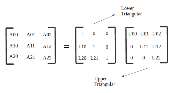
LU decomposition is a method for decomposing an matrix into a product of a lower triangular matrix
and upper triangular matrix
, as exemplified in the following figure:

is the upper triangular matrix created by the execution of the Gauss elimination process.
is the lower triangular matrix with the multipliers used in all elementary row operations in Gauss elimination. So, we’ll have
.
commonly has all the principal diagonal elements being equal to one (1) — so, we can also use it for other purposes, such as solving systems of equations.
5. LU Decomposition Using Gaussian Elimination and Finding the Determinant of a Matrix
Given a square matrix (
matrix), we may construct an upper triangular matrix
without pivoting by employing the Gaussian Elimination method. So, in this process, we’ll also get a lower triangular matrix
such that
.
Let’s take a look at this example. We will obtain and
matrices.
matrix is given as follows:
We can obtain the matrix by using the Gaussian elimination method:
R2 –(2/3) x R1 [L2,1 = 2/3]
R3 –(4/3) x R1 [L3,1=4/3]
R3 –(1/2) x R2 [L3,2 =1/2]
Therefore, is given as follows:
, in turn, is simply the multipliers from Gaussian elimination with 1s on the diagonal.
Finally, let’s calculate the determinant of matrix . As explained in Section 3, the determinant of a triangular matrix is the product of the terms on its main diagonal.
So, the determinant of a matrix that was decomposed with the LU method becomes the product of the elements on the diagonals of
and
, which are both triangular matrices:
Therefore, the determinant of matrix :
6. Implementation of LU Decomposition to Calculate Determinant of a Matrix
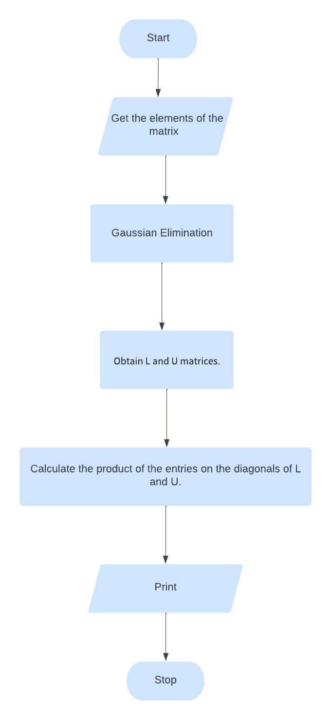
Let’s explore a flowchart that depicts the LU decomposition process to calculate a determinant of a matrix. It’s given as follows:

We’ll first apply Gaussian elimination to matrix . Gaussian elimination was explained in the previous section. Then, we’ll obtain
and
matrices. As a final step, we’ll obtain the product of the entries on the
and
main diagonals. It results in the determinant of the matrix
.
7. Complexity
We’ll discuss the time complexity of the LU decomposition technique to find matrixes’ determinants for worst-case scenarios. It’s shown in the following table:
Algorithm
Complexity
Laplace Expansion
Bareiss
LU Decomposition
The LU decomposition method is compared with two other options: Laplace expansion and the Bareiss algorithm.
Laplace expansion runs in O (n!). It’s only faster than the Bareiss algorithm and LU decomposition if the matrix is at most 5×5.
Bareiss algorithm is slightly superior to the LU decomposition for arbitrarily large matrices.
In general, the Bareiss algorithm and the LU decomposition are equivalent and vastly superior to the Laplace expansion.
8. Conclusion
In this tutorial, we learned about determinants, how to use LU decomposition to calculate the determinant of a matrix, and how to implement it. As a final step, we discussed the time complexity of this algorithm and compared it with the Bareiss algorithm and the Laplace expansion algorithm.