1. Introduction
When we design a machine learning model or try to solve any optimization problem, we aim to find the best solution. But usually, we’re using a specific dataset that fits our needs.
In that way, what happens if we apply the same solution to another problem? We can answer this question with the No Free Lunch Theorem (NFLT).
In this tutorial, we’ll explain what is defined by this principle and also give examples.
2. Definition
The NFLT was proposed back in 1997 by Wolpert and Macready. It states that no universally better algorithm can solve all types of optimization problems.
We should keep in mind that whenever we talk about optimization, we’re including but not limiting the usability of this theorem to machine learning.
Optimization problems range from artificial intelligence, and mathematical programming, to human-behavior models. So we can consider that when we aim to maximize or minimize the objective function, we’re talking about an optimization problem that follows the NFLT.
Let’s see how this theorem works and then discuss a real-life example.
2.1. Theoretical Example
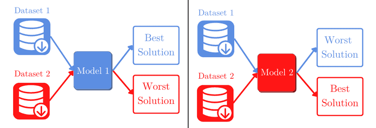
If we have dataset 1 that we used to train and design our model 1. We can reach an optimal solution for our problem. But if we use the same model, only changing to dataset 2, we probably won’t have a satisfactory result.
The same goes for the model that was developed for dataset 2. We don’t expect it to perform well on dataset 1:

This simple yet meaningful statement relies on another reinterpretation of the NFLT given by the same authors that first postulated it. Two different optimization solutions will have the same average performance if we take all possible problems.
This extends to the approaches we can implement. We can’t state that the decision trees are always better than the K-nearest neighbor algorithm.
As a first step, we should search for previous works and applications that might be similar to ours. Then, we should empirically try different learning algorithms based on our findings.
After correctly choosing the algorithm and conducting some fine-tuning, we’ll most likely be on the way to a satisfactory model.
2.2. Numerical Example
Let’s consider that we have 10 different problems. In each of them, we need to recognize words in a specific language. Due to similarities between the vocabulary, a model that performs well in one language can perform relatively well in another.
But that might not be the case for other combinations of models and problems. For this example, we’ll suppose that we have a hypothetical metric that measures the performance between 0 and 100:
Model 1
Model 2
Model 3
Model 4
Problem 1
47.96
62.85
47.12
60.56
Problem 2
58.38
59.27
61.92
74.30
Problem 3
70.27
54.81
65.19
67.48
Problem 4
54.59
56.22
64.66
62.47
Problem 5
60.05
59.37
64.42
62.01
Problem 6
65.89
49.22
57.17
66.07
Problem 7
52.26
70.87
71.64
49.42
Problem 8
46.51
60.50
68.31
67.74
Problem 9
72.99
63.79
64.33
46.10
Problem 10
71.09
63.07
35.27
43.89
Average
60.00
60.00
60.00
60.00
The NFLT states that the mean performance of all models will be the same if we consider all problems. Of course that in this example, we considered only 10 problems. But this is only for illustrative purposes.
2.3. Communication
When we want to report the outcome of our results, we need to remember the probabilistic aspect of our solution. Especially in the research environment, our inferences and predictions should be clear, so our results won’t be taken as certain.
When we reach, let’s say, an accuracy of 95%, we should pay special attention to how we communicate it. Moreover, all metrics and considerations about robustness, efficiency, and time consumption should be made with scientific rigor.
Regarding optimization problems, we should aim either to develop new algorithms or enhance existing ones for a given problem. Designing the best optimization algorithm that works for all problems is not feasible and should not be our goal.
Instead, we can choose a single problem to solve. Or even multiple problems, but keep in mind that as more generic we get, the more of the performance will be compromised.
3. Conclusion
If we’re building a machine learning model, we shout not aim to have a perfect model that will solve all problems.
The No Free Lunch Theorem comes into the light to assert that we’ll fail in this approach. Instead, we should focus on finding the best possible solution for a limited scenario and input. Or maybe enhancing a previously developed model.