锦标赛排序算法

1. Introduction

In this tutorial, we’ll discuss the tournament sort algorithm. It’s an efficient sorting algorithm that runs in linearithmic time.

2. Definition of Tournament

The algorithm borrows its name due to its similarity to elimination tournaments. In elimination tournaments, independent players or teams compete with each other. Each game is held between two players. The winner is promoted to the next round, while the loser leaves the tournament.

An example of an elimination tournament is FIFA World Cup. After the initial group stage, the best teams pass to the playoff elimination round. Each phase of playoffs reduces the number of teams by half. For example, if 16 teams have passed to the playoff, only eight teams make it to the quarters, only four teams to the semifinals, and only two teams to the final round.

The tournament can be modeled using the binary heap data structure. Specifically, MinHeap is used to decide which player passes to the next phase. The last level of MinHeap is built out of the tournament players, and each higher level is built using the level below it.

3. Tournament Sort Algorithm

There’re two versions of the tournament sort algorithm – offline and online. The offline algorithm is relatively simple and is used when the input is known beforehand and can be fully loaded into memory. The online version is more advanced and is used in memory-constrained environments or when the input comes in on the go.

The online version holds a fixed-size MinHeap in memory and fills in the bottom elements of the MinHeap as the data comes in. After the bottom level is fully filled, it builds the tournament MinHeap and sorts the data. The sorted buffer is written back to the disk or any output. After several such sorting phases, we’ll have sorted parts of the original data which then can be merged into a single sorted sequence using the -way merge approach.

We’ll cover the offline version of the tournament sort algorithm in our discussion. The steps of the offline algorithm are as follows:

1. Build the tournament MinHeap
2. Put the top element into the sorted buffer
3. Backtrack the top element to the bottom of the MinHeap and mark it as processed
4. Replay the matches along the backtracked path
5. Terminate if the top element gets marked as processed; otherwise, go to step 2

Let’s write the pseudocode for the offline tournament sort. We assume that a MinHeap node consists of the following fields:

• left – link to the left child
• right – link to the right child
• parent – link to the parent
• value – value that the node keeps
• processed – a flag indicating if the node is processed

First, we’ll introduce a couple of auxiliary operations:

algorithm PROMOTE(node):
    // INPUT
    //    node = a MinHeap node
    // OUTPUT
    //    Promotes the player associated with the node

    if node = null or node.processed:
        return null
        
    return node.value

The function below implements the logic of playing a match between two players:

algorithm MATCHRESULT(node1, node2):
    // INPUT
    //    node1 = a MinHeap node playing a match
    //    node2 = a MinHeap node playing a match
    // OUTPUT
    //    The result of the match

    promote1 <- PROMOTE(node1)
    promote2 <- PROMOTE(node2)

    if promote1 = null and promote2 = null:
        return null

    if promote1 = null:
        return promote2

    if promote2 = null:
        return promote1

    return min(promote1, promote2)

The function above accepts two MinHeap nodes, holds a match between them, and returns the result of the match. Let’s implement the backtracking logic:

algorithm BACKTRACK(r, min):
    // INPUT
    //    r = MinHeap root node
    //    min = the minimum value
    // OUTPUT
    //    Returns path p from r to a leaf node on the bottom level that equals min

    path <- an empty stack

    while r != null:
        path.push(r)
        
        if r.left != null and r.left.value = min:
            r <- r.left
        else if r.right != null and r.right.value = min:
            r <- r.right
        else:
            r.processed <- true
            r <- null
    
    return path

After we’re able to backtrack paths, we can implement the logic of replaying matches along paths:

algorithm REPLAY(path):
    // INPUT
    //    path = a sequence of MinHeap nodes
    // OUTPUT
    //    The matches along path are replayed, 
    //    the corresponding nodes are updated,
    //    and the new minimum appears on top of MinHeap.

    while path is not empty:
        node <- path.pop()

        if node.parent = null:
            break

        node.parent.value <- MatchResult(node.parent.left, node.parent.right)

Before implementing the sorting logic, let’s write the MinHeap build function:

algorithm BUILD(input):
    // INPUT
    //    input = an array of elements
    // OUTPUT
    //    The root of the built Tournament MinHeap

    nodes <- array of nodes of size input.size

    for i <- 1 to input.size:
        node <- initialize a new node
        node.value <- input[i]
        node.left <- null
        node.right <- null
        node.processed <- false
        nodes[i] <- node

    count <- nodes.size

    while count > 1:
        j <- 1

        for i <- 1, 3, 5, ..., count:
            node <- new node
            node.left <- nodes[i]
            nodes[i].parent <- node

            if i + 1 <= count:
                node.right <- nodes[i + 1]
                nodes[i + 1].parent <- node

            node.processed <- false
            node.value <- MATCHRESULT(nodes[i], nodes[i + 1])
            nodes[j] <- node

            j <- j + 1

        count <- j - 1

    return nodes[1]

Finally, we can implement the offline tournament sort algorithm:

algorithm TOURNAMENTSORT(input):
    // INPUT
    //    input = array of elements
    // OUTPUT
    //    output = array which is the sorted version of input

    root <- BUILD(input)
    output <- initialize a 1-indexed array of size input.size
    index <- 1
    
    while root.processed = false:
        output[index] <- root.value
        index <- index + 1
        path <- BACKTRACK(root, root.value)
        REPLAY(path)
    
    return output

4. Tournament Sort Algorithm Demonstration

Let’s build the tournament MinHeap step by step. Initially, we have eight elements to be sorted, and we add them to the last level of MinHeap:

The next level is built using the level below it by holding games between consecutive elements. In the games, elements with less value win. Out of eight elements, only four make it to the next level:

The next level is built in the same way. This time only two elements pass to the next level:

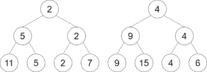
We have only two elements left. The winner takes the top of the heap.

Now, we can start taking the sorted sequence of elements out of the MinHeap. The top element is the first element in the sorted sequence:

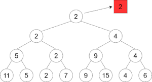
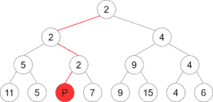
It’s time to backtrack the top element to the bottom of the heap. We mark the backtracked element with value, making it an already processed element. The processed elements don’t take part in the algorithm anymore. If both children of a node are processed, then we mark the node as processed as well:

After backtracking, we replay the matches along the backtracked path. When an element doesn’t have a rival for the current match, it immediately passes to the next level. In our case, the element with value 7 passes to the next level as its previous rival is already processed. After replaying all the matches along the path, the element with value 4 takes the top of the heap:

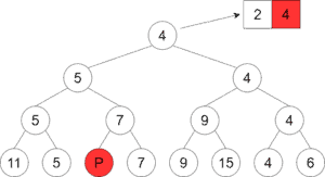
We continue the process of copying the top element to the sorted buffer, backtracking it to the bottom of the heap, and replaying the matches along the backtracked path. The algorithm terminates when the top element of the heap is marked as processed.

After repeating the process several times, we get the last element added to the sorted buffer:

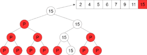
The algorithm backtracks 15 to the bottom and marks it as processed:

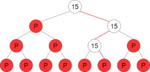
Finally, the matches along the backtracked path are replayed:

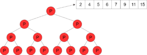
We’re done now, the top element is marked as processed, and the buffer contains the original elements in the sorted order.

Note that it’s not mandatory for the input elements count to be a power of two. Below is the tournament MinHeap for eleven elements:

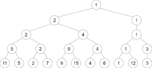
Though the heap isn’t ideally symmetric, the algorithm is the same. The time complexity isn’t affected either.

5. Complexity Analysis

The complexity of the tournament sort algorithm is linearithmic, i.e., , where is the number of elements to sort. Actually, it takes time to build the tournament MinHeap. Each element backtrack and each replay takes time. Overall, we perform backtracks and replays, so the complexity of the algorithm is .

6. Conclusion

In this tutorial, we’ve discussed the tournament sort algorithm. It’s inspired by elimination tournaments and is an efficient sort algorithm. Besides, it can be used in memory-constrained environments.