1. 简介
在图论中,最短路径问题指的是在图中寻找两个顶点之间的路径,使得路径上所有边的权重之和最小。我们可以通过 Dijkstra 算法 和 Uniform-Cost 搜索算法 来解决这类问题。
本文将介绍这两种算法的基本实现方式,并对它们在单源最短路径和单对最短路径问题中的表现进行对比分析。
2. Dijkstra 算法概述
Dijkstra 算法适用于带权有向图,且边权值为非负数。它从一个源点 s 出发,计算出到图中所有其他顶点的最短路径。
算法流程如下:
algorithm Dijkstra(G, s):
    // INPUT
    //     G = weighted directed graph (G = (V, E))
    //     s = the source vertex
    // OUTPUT
    //     dist = the shortest paths' weights from s to all vertices

    for v in V:
        dist[v] <- +infinity
    dist[s] <- 0
    Q <- empty vertex set
    for v in V:
        add v to Q with key dist[v]

    while Q is not empty:
        u <- the vertex in Q with smallest dist[u]

        remove u from Q
        visited[u] <- true
        if dist[u] == +infinity:
            break

        for v in Adj(u) and not visited[v]:
            dist <- dist[u] + w(u, v)
            if dist < dist[v]:
                dist[v] <- dist
                update Q for vertex v

    return dist
该算法使用优先队列(如最小堆)来维护顶点集合 Q,每次取出当前距离最小的顶点进行松弛操作。
时间复杂度为:✅ **O((|V| + |E|) log |V|)**,其中 |V| 是顶点数,|E| 是边数。
3. 单对最短路径的 Dijkstra 实现
当我们只需要从源点 s 到目标点 d 的最短路径时,可以对 Dijkstra 做如下优化:
- 一旦取出顶点
u == d,即可终止循环 - 使用
prev[]数组记录路径前驱,用于构建完整路径
伪代码如下:
algorithm DijkstraPair(G, s, d):
    // INPUT
    //     G = (V, E) = a weighted directed graph
    //     s = the source vertex
    //     d = the destination vertex
    // OUTPUT
    //     The list of vertices on the shortest path between s and d

    for v in V:
        dist[v] <- +infinity
    dist[s] <- 0
    Q <- empty vertex set
    for v in V:
        add v to Q with key dist[v]

    while Q is not empty:
        u <- find the vertex in Q with smallest dist[u]
        remove u from Q
        if u = d:
            break
        visited[u] <- true
        if dist[u] = +infinity:
            break

        for v in Adj(u) and not visited[v]:
            dist <- dist[u] + w(u, v)
            if dist < dist[v]:
                dist[v] <- dist
                update Q for vertex v
                prev[v] <- u

    return buildPath(s, d, prev)
路径构建函数:
algorithm buildPath(s, d, prev):
    path <- create an empty list
    v <- d
    while v != s:
        insert v at the front of path
        v <- prev[v]
    insert s at the front of path

    return path
4. Uniform-Cost 搜索算法
Uniform-Cost 是一种基于最佳优先搜索(Best-First Search)的变体,每次选择从起点出发路径代价最小的顶点进行扩展。
它与 Dijkstra 的主要区别在于:
- 初始化时只将源点加入队列
- 在扩展过程中动态加入新发现的顶点
- 更适合处理隐式图(如状态空间搜索)
4.1 流程图与伪代码
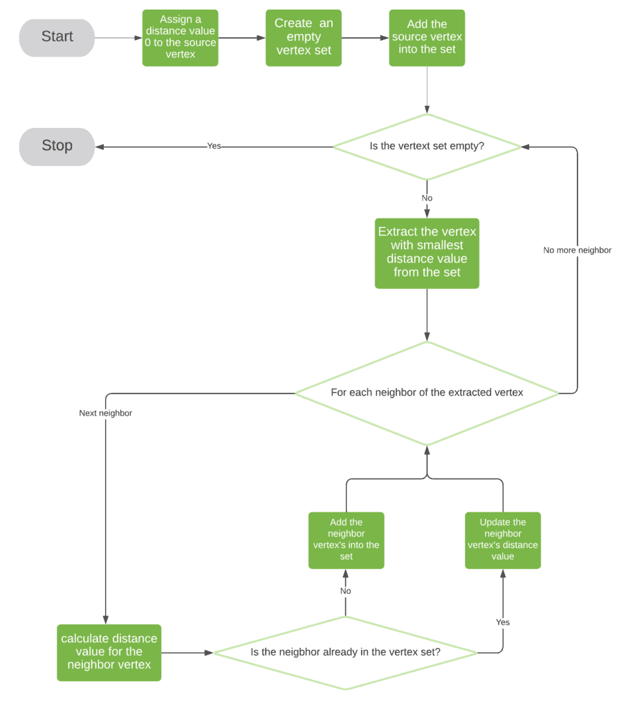
伪代码如下:
algorithm UniformCost(G, s):
    // INPUT
    //     G = (V, E) = a weighted directed graph
    //     s = the source vertex
    // OUTPUT
    //     dist = the shortest paths' weights from s to all vertices

    dist[s] <- 0
    Q <- create an empty vertex set
    add s to Q with key dist[s]

    while Q is not empty:
        u <- find the vertex in Q with smallest dist[u]

        remove u from Q

        for v in Adj(u):
            dist <- dist[u] + w(u, v)
            if v in Q:
                if dist < dist[v]:
                    dist[v] <- dist
                    update Q for vertex v
            else:
                dist[v] <- dist
                add v to Q with key dist[v]

    return dist
4.2 单对最短路径实现
同样可以扩展为单对最短路径问题:
algorithm UniformCostPair(G, s, d):
    // INPUT
    //     G = (V, E) = a weighted directed graph
    //     s = the source vertex
    //     d = the destination vertex
    // OUTPUT
    //     The path from s to d

    dist[s] <- 0
    Q <- create an empty vertex set
    add s to Q with key dist[s]

    while Q is not empty:
        u <- find the vertex in Q with smallest dist[u]

        remove u from Q
        if u = d:
            break

        for v in Adj(u):
            dist <- dist[u] + w(u, v)
            if v in Q:
                if dist < dist[v]:
                    dist[v] <- dist
                    prev[v] <- u
                    update Q for vertex v
            else:
                dist[v] <- dist
                add v to Q with key dist[v]
                prev[v] <- u

    return buildPath(s, d, prev)
5. 两种算法对比
| 特性 | Dijkstra 算法 | Uniform-Cost 搜索 |
|---|---|---|
| 初始化 | 所有顶点加入队列 | 只加入源点 |
| 内存需求 | 高(需存整个图) | 低(只存必要顶点) |
| 运行时间 | 较慢(因内存开销) | 较快 |
| 图类型支持 | 显式图 | 显式图 + 隐式图 |
| 不可达顶点 | dist[v] = +∞ | dist[v] 不存在 |
主要区别
- ✅ 初始化方式不同:Dijkstra 一次性将所有顶点加入优先队列;Uniform-Cost 动态加入
- ✅ 适用图类型不同:Dijkstra 仅适用于显式图;Uniform-Cost 适用于显式和隐式图
- ❌ 内存效率:Dijkstra 占用更高,尤其在大规模图中表现不佳
- ⚠️ 性能表现:虽然时间复杂度相同,但实际运行中 Uniform-Cost 因为内存效率更高,通常更快
6. 总结
Dijkstra 和 Uniform-Cost 都能用于解决最短路径问题,并且在理论上具有相同的时间复杂度。但在实际应用中:
- ✅ Uniform-Cost 更适合大规模图或隐式图场景
- ✅ Dijkstra 更适合图结构已知且内存充足的情况
- ⚠️ 对于单对最短路径问题,Uniform-Cost 通常表现更优
因此,在选择算法时,应根据图的规模、是否已知、内存限制等因素综合判断。