A Geometric Interpretation of Cramer’s Rule

1. Introduction

How can we solve a system of linear equations? We can use methods such as Cramer’s rule or Gaussian elimination. While the latter is more efficient for larger systems, the former is often used when the determinant can be easily computed. Another advantage of Cramer’s rule is its educational aspect. When teaching or learning linear algebra, this concept helps to illustrate the importance of determinants in solving linear systems.

In this tutorial, we’ll review how Cramer’s rule works and how we can interpret its results geometrically.

2. Cramer’s Rule

Let’s consider a simple example of a system of linear equations in two dimensions, keeping in mind that the same idea extends to higher-dimensional problems:

$[\begin{cases} ax + by = e \\ cx + dy = f \\ \end{cases}]$

We start solving it by computing the determinant of the left side:

$[D = \begin{vmatrix} a & b \\ c & d \end{vmatrix} = ad - bc]$

Next, we replace the first column with the right-hand side:

$[D_x = \begin{vmatrix} e & b \\ f & d \end{vmatrix} = ed - bf]$

Then, we do the same with the second column:

$[D_y = \begin{vmatrix} a & e \\ c & f \end{vmatrix} = af - ec]$

Finally, we obtain the values for and that solve the system as follows:

$[x = \frac{D_x}{D} \textrm{ and } y = \frac{D_y}{D}]$

2.1. Numerical Demonstration

To demonstrate, we’ll use the following linear system:

$[\begin{cases} 3x + y = 5 \\ 2x + 3y = 8 \\ \end{cases}]$

We can solve it using Cramer’s rule:

$[x = \frac{D_x}{D} = \frac{7}{7} = 1 \textrm{ and } y = \frac{D_y}{D} = \frac{14}{7} = 2]$

Is there a way to obtain the same result using a geometric interpretation of this rule?

3. Geometric Interpretation

First, let’s review the intuition behind transformations and their geometric interpretation.

3.1. Geometric Transformations and Systems of Linear Equations

A geometric transformation maps points (vectors) from the input space to vectors in the output space. Here, we’ll consider the case where the two spaces are equal and two-dimensional.

Let our transformation be:

$[T= \begin{bmatrix} a & b \\ c & d \end{bmatrix} \qquad a,b,c,d \in R]$

We assume that maps each input point to only one output point and vice versa, that for each point in a plane, only one is mapped into it.

Applying to a vector [x, y] , we get a new vector [e, f] . Algebraically, this mapping corresponds to the system of linear equations in Section 2:

$[\begin{bmatrix} a & b \\ c & d \end{bmatrix} \begin{bmatrix} x \\ y \end{bmatrix} = \begin{bmatrix} e \\ f \end{bmatrix}]$

So, we can interpret the system as the task of finding the unknown vector that transformation maps into a known vector .

3.2. Visualization of Geometric Transformations

Transformation can skew and translate vectors depending on the actual values of a, b, c, d :

transformation

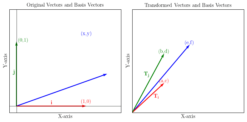
We can see that the basis vectors have changed. So, the area they span has also changed:

spanned areas

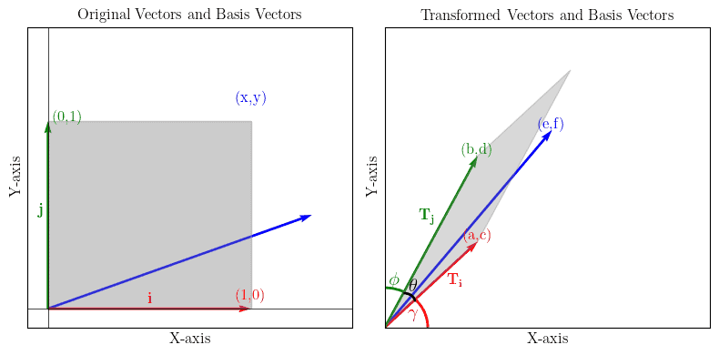
We had a unitary square that became a parallelogram stretched by a factor equal to the determinant of . Let’s verify that.

We know that the cross-product between two vectors gives the area between them. So, we can compute the new area as:

$[NewArea = \lVert \mathbf{Ti} \rVert \lVert \mathbf{Tj} \rVert \left|\sin(\theta)\right|]$

Then, we can compute $\theta$ with trigonometry:

$[\theta = 90^{\circ} - \gamma - \phi]$

where

$[\gamma = tg^{-1}\left(\frac{c}{a}\right) \qquad \phi =tg^{-1}\left(\frac{b}{d}\right)]$

If we replace the magnitude of the transformed basis vectors, we finally obtain:

$[NewArea = \sqrt{a^2 + c^2} \sqrt{b^2 + d^2} (\left|\sin(\theta)\right| )]$

If we consider our previous example, we have $a=3, b=1, c=2, \textrm{ and } d=3$ which gives us $\theta = 37.875^{\circ}$ and:

$[NewArea = (\sqrt{3^2 + 2^2}) (\sqrt{1^2 + 3^2}) (\left|\sin(37.875^{\circ})\right| ) = 7]$

This is precisely the determinant we calculated before using Cramer’s rule. So, the unitary square gets scaled by a factor of det(T) .

3.3. Geometric Solving

Next, let’s draw a parallelogram formed by the unknown vector and the unitary basis vector $\mathbf{i}$ before transformation:

beforeT

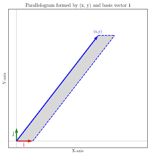
We know that the basis vector is unitary, and the height of the parallelogram is . So, we can compute its area as:

$[Area = 1 \cdot y]$

Although it’s an area, we should maintain the sign of . So, a negative yields a negative area.

After applying , the area doesn’t remain the same. As we know, it gets scaled by the determinant of . So, in the transformed space, we have:

$[NewArea = det(T) \cdot y]$

and it holds that:

$[y = \frac{NewArea}{det(T)}]$

We can also visualize the transformation and check the parallelogram formed by $\mathbf{Ti}$ and [e,f] :

transformed_vector

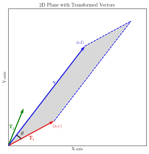
At this point, we can derive a formula to compute the new area similarly to what we did in the previous section. So we have that:

$[NewArea = (\sqrt{a^2 + c^2}) (\sqrt{e^2 + f^2}) (\left|\sin(\theta)\right| )]$

To compute the angle $\theta$ between two vectors $\mathbf{Ti}$ and $\mathbf{v}$ , we use the dot product :

$[\mathbf{Ti} \cdot \mathbf{v} = |\mathbf{Ti}| \times |\mathbf{v}| \times \cos(\theta)]$

Solving for $\theta$ , we get:

$[\theta= \cos^{-1}\left(\frac{\mathbf{Ti} \cdot \mathbf{v}}{|\mathbf{Ti}| \times |\mathbf{v}|}\right)]$

The procedure is similar for . The only difference is that we consider the parallelogram formed by the unknown vector and the transformed basis vector $\mathbf{Tj}$ .

4. Example

Let’s apply this to our initial example:

$[\begin{bmatrix} 3 & 1 \\ 2 & 3 \end{bmatrix} \begin{bmatrix} x \\ y \end{bmatrix} = \begin{bmatrix} 5 \\ 8 \end{bmatrix}]$

So, we know that with the transformation, our unknown input vector lands on the output vector . Finally, the basis vector $\mathbf{i}$ lands on the coordinates defined by the first column of . So the parallelogram becomes:

Finalexample

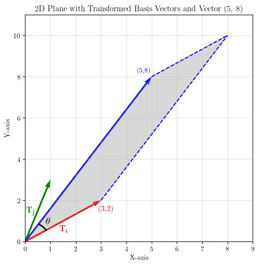
We can compute the angle with the dot product to obtain $\theta \approx 24.2^{\circ}$ .

To find , we compute the ratio of the new area and the determinant of :

$[y = \frac{NewArea}{det(T)} = \frac{(\sqrt{a^2 + c^2}) (\sqrt{e^2 + f^2}) (\left|\sin(\theta)\right| )}{\begin{vmatrix} 3 & 1 \\ 2 & 3 \end{vmatrix} } =\frac{14}{7} = 2]$

If we do the same for , we get x=1 . So, we obtained as our unknown vector, which is identical to the result we got with Cramer’s rule.

5. Conclusion

In this article, we provided a geometrical interpretation of Cramer’s rule. We leverage that a transformation in two-dimensional space stretches all the areas by a factor equal to the determinant of this transformation’s matrix. The same reasoning extends to higher dimensions. In a three-dimensional space, the determinant of the transformation represents the factor by which volumes are scaled, and so on.

Persistence

REST

Security