1. 简介
在本文中,我们将深入探讨德布鲁因序列(de Bruijn Sequence)这一数学概念。 我们会解释它是什么、它的实际应用场景,以及如何通过算法生成它。
2. 什么是德布鲁因序列?
德布鲁因序列是一种数学结构。给定一个包含 k 个字符的字母表,阶数为 n 的德布鲁因序列是一个连续序列,其中包含了这个字母表中所有长度为 n 的字符串,且每个字符串恰好出现一次。
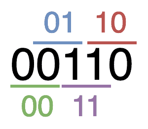
举个简单的例子:如果我们使用二进制字母表(0 和 1),阶数为 2,那么所有长度为 2 的字符串就是 00、01、10、11。一个对应的德布鲁因序列可以是 00110。这个序列中包含了所有 4 个组合,而且每个组合只出现一次。
需要注意的是,德布鲁因序列本质上是循环的。也就是说,如果我们把序列的首尾连接起来,从任意位置开始读取长度为 n 的子串,都能得到所有可能的组合。
例如,一个阶数为 2 的二进制德布鲁因序列可以是:
如果我们把首尾连接起来,可以看作是一个无限循环的序列,比如:...001100110011001100...。
3. 德布鲁因序列的应用场景
德布鲁因序列广泛应用于多个领域,包括但不限于:
- 生物信息学(基因组拼接)
- 机器人定位
- 数据加密
- 安全攻防
- 密码破解
3.1 机器人方向识别
在机器人导航中,德布鲁因序列可用于识别摄像头的朝向。我们可以将序列打印成环形图案,围绕摄像头排列,这样摄像头只要看到其中一段子序列,就能唯一确定自己的方向。
例如,使用一个阶数为 3、字母表大小为 2 的德布鲁因序列,我们可以生成一个包含所有 8 个三位二进制数的序列。将这个序列以黑白方块形式环绕摄像头,摄像头看到的任意三个连续符号就能唯一确定方向。
✅ 优势:
- 字母表大小小(如黑白两色),仍可支持高分辨率方向识别
- 阶数为 5 时,仅需 2 个符号即可支持 32 个方向
⚠️ 扩展性:
- 若字母表增大为 3 种颜色(如红、绿、蓝),阶数为 3 就能支持 27 个方向,阶数为 5 更是支持 243 个方向
3.2 密码锁暴力破解
假设我们面对一个四位数字密码锁,密码长度为 4,输入时无需按“确认”键即可立即验证。如果我们从 0000 到 9999 逐一尝试,最多需要 40,000 次按键。
但如果我们使用德布鲁因序列,就可以大大减少输入次数。因为德布鲁因序列是连续的,每个密码都与前一个密码部分重叠,所以只需要输入长度为 10,000 + 3 = 10,003 的序列即可覆盖所有可能。
✅ 优势:
- 极大减少输入次数
- 可用于各种数字或符号组合的密码破解
4. 如何生成德布鲁因序列?
德布鲁因序列的生成可以通过图论方法实现,具体步骤如下:
4.1 构建有向图
生成所有节点:
对于阶数 n,我们生成所有长度为 n-1 的字符串作为节点。例如,二进制下阶数为 3,则节点是00,01,10,11。构建边:
每个节点连接到另一个节点,方式是:去掉当前字符串的首字符,加上一个新字符(来自字母表),形成新的节点。每条边的字符就是新添加的字符。
例如,节点 01:
- 添加字符
0→ 新节点为10 - 添加字符
1→ 新节点为11
这样我们就能构建出一个有向图。
4.2 寻找欧拉路径(Eulerian Path)
由于每个节点的入度和出度相等,因此图中一定存在一个欧拉回路(Eulerian Circuit),即可以走完所有边且不重复。
我们可以通过 Hierholzer 算法 找到这个回路,并在过程中记录每条边上的字符,最终拼接成德布鲁因序列。
4.3 Java 示例代码
✅ 生成所有节点
List<String> generateNodes(List<Character> alphabet, int order) {
    List<String> nodes = new ArrayList<>();
    for (char c : alphabet) {
        nodes.add(String.valueOf(c));
    }

    for (int i = 0; i < order - 2; i++) {
        List<String> temp = new ArrayList<>();
        for (String node : nodes) {
            for (char c : alphabet) {
                temp.add(node + c);
            }
        }
        nodes = temp;
    }

    return nodes;
}
✅ 构建图结构
Map<String, Map<Character, String>> generateGraph(List<String> nodes, List<Character> alphabet) {
    Map<String, Map<Character, String>> graph = new HashMap<>();

    for (String node : nodes) {
        Map<Character, String> edges = new HashMap<>();
        for (char c : alphabet) {
            String next = node.substring(1) + c;
            edges.put(c, next);
        }
        graph.put(node, edges);
    }

    return graph;
}
✅ 使用 Hierholzer 算法生成序列
List<String> generateSequence(Map<String, Map<Character, String>> graph) {
    List<String> sequence = new ArrayList<>();
    String start = graph.keySet().iterator().next();

    Deque<String> stack = new LinkedList<>();
    Deque<String> circuit = new LinkedList<>();

    stack.push(start);
    String current = start;

    while (!stack.isEmpty()) {
        if (!graph.get(current).isEmpty()) {
            stack.push(current);
            char edge = graph.get(current).keySet().iterator().next();
            String next = graph.get(current).get(edge);
            graph.get(current).remove(edge);
            current = next;
        } else {
            circuit.push(current);
            current = stack.pop();
        }
    }

    // 构建最终序列
    StringBuilder sb = new StringBuilder();
    for (String node : circuit) {
        sb.append(node.charAt(node.length() - 1));
    }

    return Arrays.asList(sb.toString().split(""));
}
4.4 示例图演示
我们以节点 00 开始,依次走边 0, 1, 0, 1, 1, 1, 0, 0,最终生成的序列是:
5. 小结
✅ 本文我们学习了:
- 德布鲁因序列的定义及其数学特性
- 它在机器人定位、密码破解等领域的实际应用
- 如何通过图论和 Hierholzer 算法生成德布鲁因序列
⚠️ 踩坑提醒:
- 图结构的构建要确保每个节点的边都正确无误
- 在使用 Hierholzer 算法时要注意边的删除和栈的顺序处理
德布鲁因序列虽然看起来数学味很浓,但其在工程实践中非常实用。建议读者动手实现一次生成算法,加深理解。