蝗虫优化算法（Grasshopper Optimization Algorithm）

1. 概述

优化算法在计算机科学中有着广泛的应用，其中蝗虫优化算法（Grasshopper Optimization Algorithm，GOA）是一种新兴的群体智能优化方法。它通过模拟自然界中蝗虫群体的行为来寻找问题的最优解。

本文将介绍 GOA 的基本原理、数学模型、实现步骤，并通过一个数值示例展示其求解过程。最后我们还会总结其优缺点，帮助读者全面理解这一算法。

2. 什么是蝗虫优化算法？

GOA 是一种基于群体的元启发式算法，由 Saremi 和 Mirjalili 于 2017 年提出，用于解决数值优化问题。它的灵感来源于自然界中蝗虫群体的社交行为和觅食方式。

该算法通过模拟蝗虫之间的相互作用、风向影响和重力作用，来更新每个“解”的位置，从而在搜索空间中逐步逼近最优解。

3. 蝗虫的行为特征

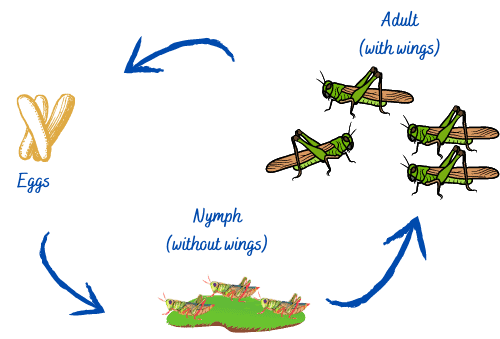
蝗虫生命周期包括三个阶段：卵、若虫和成虫。

• 卵阶段：夏季在植物附近产卵，冬季进入休眠，春季孵化
• 若虫阶段：没有翅膀，移动缓慢，逐步发育成成虫
• 成虫阶段：拥有翅膀，可进行远距离飞行和快速移动

在算法中，我们主要关注的是成虫阶段的快速移动和群体行为，这是 GOA 的核心灵感来源。

蝗虫群体觅食行为分为两个阶段：

• 探索阶段（Exploration）：广泛搜索食物来源
• 开发阶段（Exploitation）：在已知食物源附近精细搜索

这两个阶段的平衡是 GOA 算法设计的关键。

4. GOA 的数学模型

GOA 算法模拟了蝗虫的三种行为力：社交互动、重力和风向影响。每个蝗虫的位置由以下公式计算：

(1)
$$ X_i = S_i + G_i + A_i $$

其中：

• $ S_i $：与其他蝗虫的社交互动
• $ G_i $：重力影响
• $ A_i $：风向影响

在实际实现中，为增加随机性，加入随机系数：

(2)
$$ X_i = r_1 S_i + r_2 G_i + r_3 A_i $$

其中 $ r_1, r_2, r_3 \in [0,1] $

4.1 社交互动力

社交互动是 GOA 的核心部分，表示为：

(3)
$$ S_i = \sum_{j=1}^{N} s(d_{ij}) \hat{d_{ij}}, \quad i \neq j $$

其中 $ d_{ij} = |x_j - x_i| $ 是蝗虫之间的距离，$ \hat{d_{ij}} = \frac{x_j - x_i}{d_{ij}} $ 是单位向量。

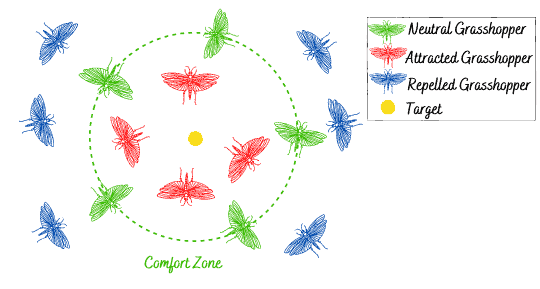
函数 $ s(r) $ 表示吸引力和排斥力的强度：

(4)
$$ s(r) = f e^{-r/l} - e^{-r} $$

其中：

• $ f $：吸引力强度
• $ l $：吸引力长度尺度

当蝗虫之间距离在 [0, 2.079] 范围内时，表现为排斥力；在 2.079 处为舒适区；超过 2.079 后表现为吸引力。

4.2 重力力

重力作用方向朝向地球中心：

(5)
$$ G_i = -g \hat{e_g} $$

其中 $ g $ 是重力常数，$ \hat{e_g} $ 是单位向量。

4.3 风向力

风向对蝗虫的移动有显著影响，特别是在成虫阶段：

(6)
$$ A_i = u \hat{e_w} $$

其中 $ u $ 是风漂移常数，$ \hat{e_w} $ 是风向单位向量。

4.4 蝗虫位置更新公式

综合以上三种力，最终的蝗虫位置更新公式如下：

(7)
$$ X_i = \sum_{j=1}^{N} s(|x_j - x_i|) \frac{x_j - x_i}{d_{ij}} - g \hat{e_g} + u \hat{e_w}, \quad i \neq j $$

为了防止蝗虫过早陷入局部最优，GOA 引入了一个衰减系数 $ c $ 来动态调整社交互动的范围：

(8)
$$ X_i^d = c \left( \sum_{j=1}^{N} \frac{UB_d - LB_d}{2} s(|x_j^d - x_i^d|) \frac{x_j - x_i}{d_{ij}} \right) + \text{Best Solution} $$

其中 $ c $ 是一个随迭代次数递减的系数：

(9)
$$ c = c_{max} - iter \cdot \frac{c_{max} - c_{min}}{Max_{iter}} $$

5. GOA 算法步骤

以下是 GOA 算法的伪代码实现：

algorithm GrasshopperOptimizer(iter, c_max, c_min, l, f, n, Max_iter):
    // 参数说明：
    // c_max, c_min：c 的最大最小值
    // l：吸引力长度尺度
    // f：吸引力强度
    // n：蝗虫数量
    // Max_iter：最大迭代次数
    
    // 初始化蝗虫种群
    grasshoppers = initialize n solutions (X_1, X_2, ..., X_n)
    
    // 计算适应度
    Compute fitness for each grasshopper
    
    // 找出当前最优解
    bestSolution = findBest(grasshoppers)
    
    iter = 0
    while iter < Max_iter:
        update c using equation (9)
        
        for grasshopper in grasshoppers:
            normalize distance between [1, 4]
            update position using equation (8)
            check boundaries
            
        update bestSolution if found better one
        iter += 1
        
    return bestSolution

时间复杂度分析

GOA 的时间复杂度主要取决于种群数量和迭代次数：

$$ O(n \times Max_{iter}) $$

6. 数值示例

我们通过一个简单的优化问题来演示 GOA 的执行过程。

6.1 初始化参数

我们设定如下参数：

参数	值	说明
Max_iter	9	最大迭代次数
c_max	1	c 的最大值
c_min	0.00004	c 的最小值
LB	-5	下界
UB	5	上界
d	2	维度

初始化蝗虫种群：

序号	X(1)	X(2)
1	3.1472	1.3236
2	4.0579	-4.0246
3	-3.7301	-2.2150
4	4.1338	0.4688

6.2 计算适应度值

我们使用如下适应度函数：

$$ Fitness = 4x_1^2 - 2.1x_1^4 + \frac{1}{3}x_1^6 + x_1x_2 - 4x_2^2 + 4x_2^4 $$

计算结果如下：

序号	X(1)	X(2)	Fitness
1	3.1472	1.3236	166.9550
2	4.0579	-4.0246	1953.1
3	-3.7301	-2.2150	631.9194
4	4.1338	0.4688	1119.6

当前最优解为 166.9550。

6.3 归一化距离

根据公式 (10) 和 (11)：

$$ c = 1 - 2 \cdot \frac{1 - 0.00004}{9} \approx 0.80001 $$

计算各蝗虫之间的归一化距离：

序号	Distance(1)	Distance(2)
1	0.0058	-0.1533
2	-0.0756	0.13648
3	0.1565	-0.0275
4	-0.0867	-0.0106

6.4 更新位置

根据公式 (8) 更新各蝗虫的新位置：

序号	X(1)	X(2)
1	3.1519	1.2009
2	3.0867	1.4328
3	3.1472	1.3236
4	3.0778	1.3151

6.5 重新计算适应度

更新后计算新的适应度值：

序号	Fitness
1	165.6341
2	148.8582
3	221.6412
4	141.9027

发现最优解更新为 141.9027。

6.6 全局最优解更新

继续迭代，直到达到最大迭代次数。最终得到最优解为：

$$ \text{Best Global Solution} = 124.3374 $$

7. GOA 的优缺点

优点 ✅	缺点 ❌
能有效解决无约束和有约束的全局优化问题	易陷入局部最优
实现简单	收敛速度较慢
精度高	对参数敏感
能找到高质量解	初始种群影响大

8. 总结

GOA 是一种基于蝗虫群体行为的新型元启发式优化算法，具有良好的全局搜索能力。通过模拟蝗虫的社交行为、风向影响和重力作用，GOA 在复杂优化问题中表现出了不错的性能。

虽然它在某些场景下存在收敛速度慢和易陷入局部最优的问题，但通过参数调整和改进策略，可以在一定程度上缓解这些问题。

✅ 建议：对于需要高精度、全局搜索能力强的优化任务，GOA 是一个值得尝试的算法。
⚠️ 注意：在实际使用中，需结合问题特点合理设置参数，并考虑引入局部搜索机制以提高收敛速度。