1. 引言
本文将回顾主成分分析(PCA),并介绍如何在使用 PCA 时选择最佳的主成分数量。
最后,我们会以一个流行的机器学习数据集为例,演示 PCA 的实际应用。
2. 降维简介
降维是指将数据从高维空间转换到一个低得多的新空间中的过程。在信号处理领域中,这与数据压缩密切相关。
在机器学习中,降维通常用于加快模型训练速度。此外,某些情况下,减少数据维度可以过滤掉噪声特征,从而提升模型的准确率。降维在数据可视化方面也十分有用,尤其是将数据降至二维或三维后,可以通过图形直观地展示高维数据并提取关键信息。
3. PCA 概述
✅ PCA 是最流行的降维技术之一。
在 PCA 中,压缩和还原过程是通过线性变换实现的。其核心思想是找到一种线性变换方式,使得在数据集上的均方误差最小。
假设我们有 $ M $ 个特征向量 $ \mathbf{x}_1, \dots, \mathbf{x}_M $,它们属于 $ \mathbb{R}^D $ 空间。我们使用一个大小为 $ N \times D $ 的实矩阵 $ T $(其中 $ N < D $)进行线性变换:
$$
\mathbf{y} = T \mathbf{x}
$$
这个变换将数据压缩到低维空间。
随后,使用另一个大小为 $ D \times N $ 的矩阵 $ U $,我们可以从压缩后的 $ \mathbf{y} $ 重建原始向量:
$$
\tilde{\mathbf{x}} = U \mathbf{y}
$$
PCA 的目标就是找到这样的 $ T $ 和 $ U $,使得重建误差最小,即求解如下优化问题:
$$ \operatorname{argmin}{(T , U)} \sum{i=1}^{M}\left|\mathbf{x}{i}- U T \mathbf{x}{i} \right|_{2}^{2} $$
数学上可以证明:
- 如果 $ T $ 是解,那么 $ U = T^\top $
- $ T $ 的列向量对应于数据的协方差矩阵的特征向量
因此,PCA 的核心是计算协方差矩阵的特征向量(即主成分)并按对应特征值大小排序。
协方差矩阵定义如下:
$$ C =\frac{1}{M-1} \sum_{i=1}^{M}\left(\mathbf{x}i- \boldsymbol{\mu}{x} \right)\left(\mathbf{x}i-\boldsymbol{\mu}{x} \right)^{\top} $$
其中:
$$ \boldsymbol{\mu}{x} = \frac{1}{M} \sum{i=1}^{M} \mathbf{x}_i $$
最终,PCA 的压缩矩阵 $ T $ 可以表示为:
$$ T = \left[\begin{array}{c} \mathbf{u}_1 \cdots \mathbf{u}_N \end{array}\right] $$
其中 $ \mathbf{u}_1, \dots, \mathbf{u}_N $ 是按特征值从大到小排序的特征向量。
4. 如何选择主成分数量?
每个特征值 $ \lambda_i $ 表示数据在对应主成分方向上的方差。因此,特征值越小,该方向上的信息越少,可以被舍弃。
我们常用 解释方差比(explained variance ratio) 来衡量每个主成分的重要性:
$$ \text{explained variance ratio of the i-th component} = \frac{\lambda_i}{\sum^D_{j=1} \lambda_j} $$
将前 $ N_{pc} $ 个主成分的解释方差比相加,就得到 累计解释方差(cumulative explained variance):
$$ \text{cumulative explained variance} = \frac{\sum^{N_{pc}}{j=1}\lambda_j}{\sum^D{j=1} \lambda_j} $$
✅ 推荐策略:选择使得累计解释方差超过某个阈值(如 95%)的最小主成分数。
⚠️ 注意: 阈值选择需根据实际场景调整。例如,图像识别任务可能需要更高累计方差(如 99%),而其他任务 90% 可能已足够。
5. 示例:MNIST 数据集上的 PCA 应用
下面我们使用 Python 的 scikit-learn 库对 MNIST 数据集进行 PCA 演示。
5.1 加载并预处理数据
import numpy as np
from keras.datasets import mnist

(x_train, y_train), (x_test, y_test) = mnist.load_data()
x_train = x_train.reshape(-1, 28*28) / 255.0  # 归一化到 [0, 1]
5.2 执行 PCA 并计算累计解释方差
from sklearn.decomposition import PCA

pca = PCA()
pca.fit(x_train)
cumsum = np.cumsum(pca.explained_variance_ratio_)
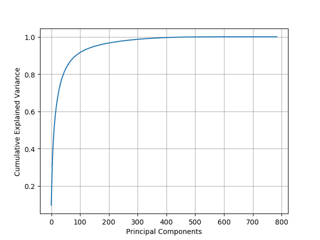
5.3 可视化累计解释方差曲线
绘制累计解释方差随主成分数量变化的曲线,观察“肘部”拐点:
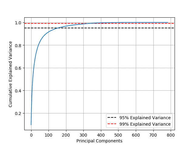
5.4 选择保留 95% 方差的主成分数量
d = np.argmax(cumsum >= 0.95) + 1
print(f"保留95%方差需要 {d} 个主成分")
输出:保留95%方差需要 150 个主成分
这意味着我们可以将 784 维的图像数据压缩到 150 维,仅保留原始数据大小的 19%!
5.5 如果保留 99% 的方差呢?
d = np.argmax(cumsum >= 0.99) + 1
print(f"保留99%方差需要 {d} 个主成分")
输出:保留99%方差需要 330 个主成分
此时压缩后的数据为原始大小的 42%。
6. 小结
本文回顾了主成分分析(PCA)的基本原理,并介绍了如何通过累计解释方差选择合适的主成分数量。
我们通过 MNIST 数据集演示了如何使用 scikit-learn 实现 PCA,并展示了不同主成分数量对数据压缩效果的影响。
✅ 关键点总结:
- PCA 是一种基于协方差矩阵特征分解的线性降维方法
- 主成分按特征值从大到小排序
- 通过累计解释方差选择主成分数是一个常用且有效的方法
- 95% 是一个常见的累计方差阈值,但需根据具体任务调整
如果你正在处理高维数据,PCA 是一个值得尝试的预处理工具,能有效提升训练效率和模型表现。