1. 概述
在本教程中,我们将深入讲解 线性探测法(Linear Probing),这是一种用于解决哈希表中哈希冲突的经典方法。哈希表作为高效的数据结构,通过将键映射到索引来实现快速的插入与查找操作。但不同键可能通过哈希函数映射到相同的索引上,从而产生冲突。
线性探测是一种开放寻址策略,它通过线性扫描的方式寻找下一个可用的空槽位来解决冲突。我们不仅会演示如何使用线性探测进行插入操作,还会介绍它在查找操作中的实现。
2. 什么是线性探测?
线性探测(Linear Probing)是用于解决哈希冲突的一种策略。当两个不同的键哈希到相同的索引时,线性探测会从该索引开始,依次向后查找直到找到一个空位,然后将键插入该位置。
查找操作也遵循类似的逻辑:从哈希值对应的索引出发,线性扫描直到找到目标键或遇到空位为止。
举个例子:
我们有如下一组键 A 和哈希函数 h:
A = {40, 310, 74, 9, 2}
h(a) = {1, 3, 4, 5, 3}  ∀a ∈ A
插入键 2 时,其哈希值为 3,但索引 3 已被占用。于是我们从 3 开始依次往后查找空位:
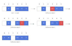
最终发现索引 0 是第一个空位,于是将 2 插入到索引 0。
⚠️ 注意:如果哈希表已满,线性探测应能及时终止查找,避免无限循环。
3. 线性探测的插入逻辑
线性探测插入操作的核心在于:
- 从哈希值对应的索引开始
- 线性向后查找空槽
- 如果遇到空槽,则插入键
- 如果遍历完整个表仍未找到空槽,则插入失败
下面是插入操作的伪代码实现:
algorithm LinearProbingInsert(hash_table, table_length, key, hash_value):
    // INPUT
    //    hash_table = the hash table to insert the key into
    //    table_length = the length of the hash table
    //    key = the key to insert
    //    hash_value = the initial hash value for the key
    // OUTPUT
    //    true if the key is successfully inserted, false if there is no space to insert the key

    index <- hash_value
    first_scan <- true

    while isEmpty(hash_table, index) = false:
        index <- (index + 1) mod table_length
        if index = hash_value and first_scan = false:
            return false
        first_scan <- false

    hash_table[index] <- key
    return true
✅ 插入成功时返回 true,表满无法插入时返回 false。
4. 线性探测的查找逻辑
查找操作与插入类似,也是从哈希值对应的索引开始,依次线性扫描,直到找到目标键或遇到空槽(说明该键不存在)。
伪代码如下:
algorithm LinearProbingSearch(hash_table, table_length, key, hash_value):
    // INPUT
    //    hash_table = the hash table to search in
    //    table_length = the length of the hash table
    //    key = the key to search for
    //    hash_value = the hash value of the key
    // OUTPUT
    //    the index where the key is found, or -1 if the key is not in the hash table

    index <- hash_value
    first_scan <- true

    while hash_table[index] != key:
        index <- (index + 1) mod table_length
        if index = hash_value and first_scan = false:
            return -1
        first_scan <- false

    return index
✅ 找到键返回其索引,否则返回 -1。
5. 时间复杂度分析
理想情况下,一个设计良好的哈希函数可以使得插入和查找接近 O(1) 的时间复杂度。
但由于线性探测需要在发生冲突时线性扫描下一个空位,最坏情况下(表几乎满),每次插入或查找都可能需要扫描整个表。
因此,线性探测的最坏时间复杂度为:
✅ **O(n)**,其中 n 为哈希表长度
虽然时间复杂度不如链式哈希(chaining)理想,但线性探测实现简单,空间利用率高,在某些场景下仍然有其优势。
6. 小结
线性探测是一种经典的哈希冲突解决策略,适用于开放寻址法(Open Addressing)的哈希表实现。它的核心思想是:
- 插入时,从哈希值出发线性查找空位
- 查找时,从哈希值出发线性查找目标键
- 避免死循环,必须在扫描一圈后终止
虽然其最坏时间复杂度为 O(n),但在实际应用中,**如果哈希表负载因子控制得当,性能仍可非常接近 O(1)**。
✅ 优点:
- 实现简单
- 空间利用率高
- 适合缓存友好的场景
❌ 缺点:
- 容易产生聚集(clustering),影响性能
- 负载因子过高时效率下降明显
线性探测法虽然简单,但在某些场景下仍被广泛使用,例如 Java 中的 ThreadLocalMap 就使用了线性探测法来处理哈希冲突。