1. 引言
隐马尔可夫模型(Hidden Markov Model, HMM)是一种经典统计模型,自20世纪60年代提出以来,被广泛应用于多个科学领域,至今仍被广泛用于处理序列建模任务。
最初用于语音识别,后来被用于词性标注、时间序列分析、基因预测、交通优化等多个领域。
✅ HMM之所以有效,是因为它基于坚实的数学原理,结构简单但具有高度通用性。
2. 模型原理
2.1. 一个猜天气的游戏
Alice和Bob每天通过电话聊天,Bob会告诉她当天做了什么活动。Alice的任务是根据这些活动推断天气情况。
简化设定如下:
- Bob的活动:散步、购物、打扫
- 天气状态:晴天、雨天
💡 核心思想:观察到的活动依赖于不可见的天气状态,天气本身遵循某种状态转移规律。
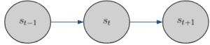
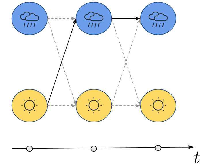
2.2. 马尔可夫性质
HMM的一个关键假设是马尔可夫性质(Markov Property):
下一状态只与当前状态有关,与更早的历史无关。
数学表达如下:
$$ p(s_{t+1} \mid s_t, s_{t-1}) = p(s_{t+1} \mid s_t) $$
图示如下:
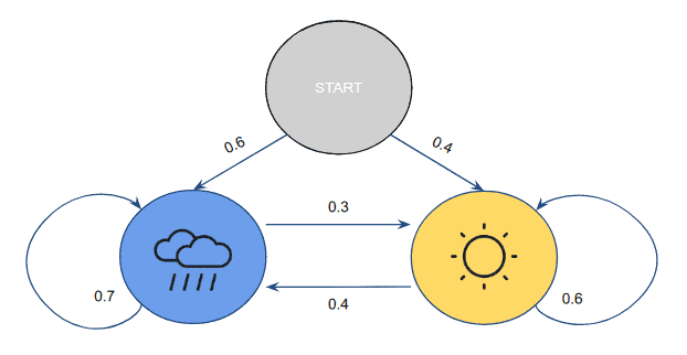
2.3. 马尔可夫链
根据Alice的经验,她可以构建一个天气状态转移的概率模型:
- 若昨天是晴天:
- 今天晴天的概率为 0.6
- 今天下雨的概率为 0.4
- 若昨天是雨天:
- 今天继续下雨的概率为 0.7
- 今天转晴的概率为 0.3
初始状态概率:
- 雨天开始:0.6
- 晴天开始:0.4
图示如下:
状态转移矩阵 A:
$$ A = \begin{bmatrix} 0.6 & 0.4 \ 0.3 & 0.7 \end{bmatrix} $$
初始概率向量 π:
$$ \pi = \begin{bmatrix} 0.4 & 0.6 \end{bmatrix} $$
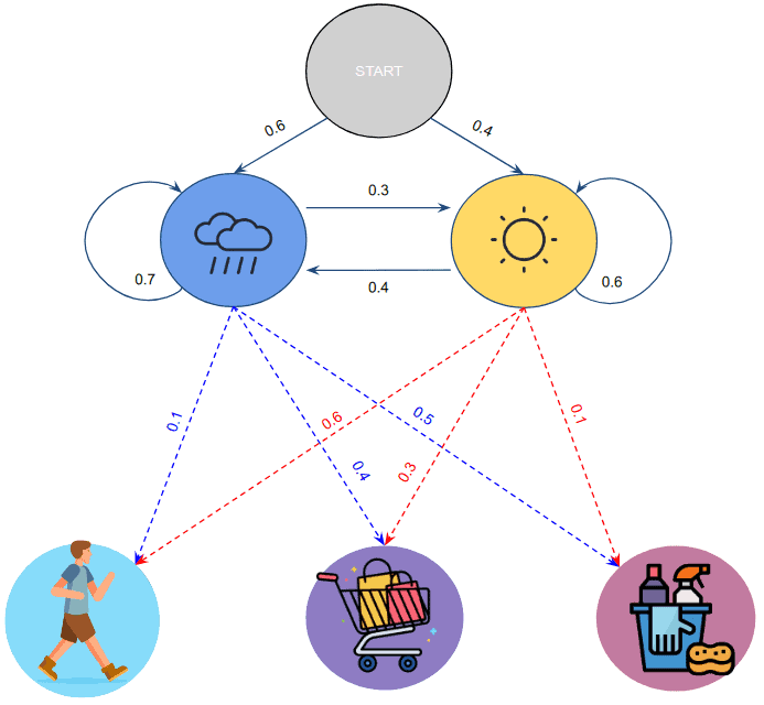
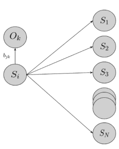
2.4. 发射概率(Emission Probabilities)
每种天气下,Bob的活动概率不同:
- 晴天:
- 散步:0.8
- 购物:0.1
- 打扫:0.1
- 雨天:
- 散步:0.1
- 购物:0.4
- 打扫:0.5
发射概率矩阵 B:
$$ B = \begin{bmatrix} 0.8 & 0.1 & 0.1 \ 0.1 & 0.4 & 0.5 \end{bmatrix} $$
图示如下:
3. 评估问题(Evaluation Problem)
我们的问题是:给定一个观察序列(如:散步、购物、打扫),这个模型生成该序列的概率是多少?
数学表达为:
$$ p(O_T \mid \theta) = ? $$
其中:
- $ O_T $:观察序列
- $ \theta $:模型参数(A、B、π)
3.1. 暴力解法
对于每个可能的状态序列 $ S_q $,计算其与观察序列的联合概率,再求和:
$$ p(O \mid \theta) = \sum_{q=1}^{Q} p(O, S_q \mid \theta) $$
但计算复杂度极高,达到 $ O(T \times N^T) $,不可行。
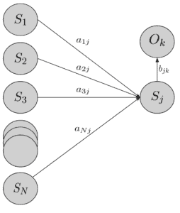
3.2. 前向算法(Forward Algorithm)
通过动态规划优化,使用前向变量 $ \alpha_t(i) $ 表示在时间 t 时处于状态 i 且观察序列匹配的概率。
定义如下:
- 初始值: $$ \alpha_1(i) = \pi_i b_i(O_1) $$
- 递归公式: $$ \alpha_{t+1}(j) = \left( \sum_{i=1}^N \alpha_t(i) a_{ij} \right) b_j(O_{t+1}) $$
最终结果:
$$ p(O_T \mid \theta) = \sum_{i=1}^N \alpha_T(i) $$
图示如下:
复杂度优化为 $ O(T \times N^2) $,大幅提升了效率。
3.3. 后向算法(Backward Algorithm)
与前向算法对称,后向变量 $ \beta_t(i) $ 表示在时间 t 时处于状态 i 且后续观察序列匹配的概率。
定义如下:
- 初始值: $$ \beta_T(i) = 1 $$
- 递归公式: $$ \beta_t(i) = \sum_{j=1}^N a_{ij} b_j(O_{t+1}) \beta_{t+1}(j) $$
图示如下:
4. 解码问题(Decoding Problem)
核心问题:给定观察序列,最可能的状态序列是什么?
4.1. Viterbi 算法
使用动态规划思想,定义变量 $ \delta_t(i) $ 表示在时间 t 时处于状态 i 且路径最优的概率,同时记录路径来源 $ \psi_t(i) $。
定义如下:
- 初始值: $$ \delta_1(i) = \pi_i b_i(O_1), \quad \psi_1(i) = 0 $$
- 递归公式: $$ \delta_t(j) = \max_{1 \le i \le N} \left[ \delta_{t-1}(i) a_{ij} \right] b_j(O_t) $$ $$ \psi_t(j) = \arg\max_{1 \le i \le N} \left[ \delta_{t-1}(i) a_{ij} \right] $$
最终通过回溯重建路径。
图示如下:
5. 总结
- HMM 是一种基于马尔可夫性质的统计模型,广泛用于序列建模。
- 包含三个核心参数:状态转移矩阵 A、发射矩阵 B、初始概率 π。
- 通过 Forward-Backward 算法可以高效评估模型生成观察序列的概率。
- Viterbi 算法可用于解码隐藏状态序列,是 HMM 实际应用的关键。
💡 踩坑提醒:不要直接暴力枚举所有状态序列,否则在实际应用中根本无法运行。一定要使用动态规划方法如 Forward 和 Viterbi 算法。
✅ HMM 的优势在于模型简洁、数学基础扎实,适合处理具有时序依赖的问题。