1. 概述
在本教程中,我们将讨论如何将两个有序数组合并为一个有序数组,并重点讲解其背后的理论思想。我们会以伪代码形式展示解决方案,而非特定编程语言实现。
我们将先定义问题并辅以示例说明,然后介绍两种不同的实现方法,最后对比它们的复杂度和适用场景。
2. 问题定义
我们有两个数组:
- 数组 A,长度为 n
- 数组 B,长度为 m
这两个数组都是升序排列的。我们的任务是将它们合并为一个新的数组 R,长度为 n + m,并且这个新数组也必须是升序排列的。
举个例子帮助理解:
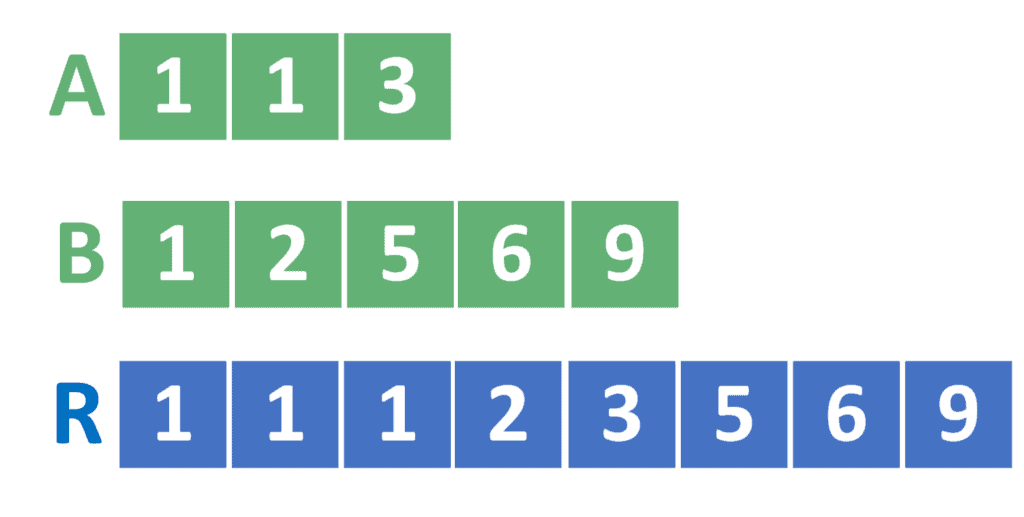
如图所示:
- A 有 3 个元素:[1, 2, 4]
- B 有 5 个元素:[1, 3, 5, 6, 7]
- 合并后 R 应有 8 个元素:[1, 1, 2, 3, 4, 5, 6, 7]
注意:
- 合并后的数组必须包含 A 和 B 的所有元素
- 元素顺序必须保持升序
3. 暴力解法(Naive Approach)
✅ 思路
将 A 和 B 的所有元素复制到新数组 R 中,然后对 R 进行排序。
✅ 示例代码
algorithm naiveMerge(A, B):
    R <- empty array of size n + m
    id <- 0

    for i <- 0 to n - 1:
        R[id] <- A[i]
        id <- id + 1

    for j <- 0 to m - 1:
        R[id] <- B[j]
        id <- id + 1

    sort(R)
    return R
⚠️ 时间复杂度
- 复制操作:O(n + m)
- 排序操作:O((n + m) * log(n + m))
- 总体复杂度:✅ O((n + m) * log(n + m))
❌ 缺点
- 没有利用 A 和 B 已排序的特性
- 效率较低,尤其当数组很大时明显慢于优化方法
4. 双指针解法(Two-Pointers Approach)
4.1 核心思想
既然 A 和 B 都是有序的,那么我们可以:
- 用两个指针 i 和 j 分别指向 A 和 B 的当前待比较元素
- 每次比较 A[i] 和 B[j],选择较小的放入结果数组 R
- 移动相应的指针继续比较,直到其中一个数组遍历完
- 最后将剩余未遍历完的数组元素直接复制到 R 的剩余位置
4.2 示例代码
algorithm twoPointersMerge(A, B):
    i <- 0
    j <- 0
    R <- empty array of size n + m

    for id <- 0 to n + m - 1:
        if j >= m:
            R[id] <- A[i]
            i <- i + 1
        else if i >= n:
            R[id] <- B[j]
            j <- j + 1
        else if A[i] <= B[j]:
            R[id] <- A[i]
            i <- i + 1
        else:
            R[id] <- B[j]
            j <- j + 1

    return R
✅ 时间复杂度
- 每个元素只被访问一次
- 总体复杂度:✅ O(n + m)
✅ 优势
- 充分利用了数组已排序的特性
- 时间效率高,适合大规模数据合并
5. 方法对比
| 方法 | 时间复杂度 | 是否利用有序特性 | 适用场景 |
|---|---|---|---|
| 暴力解法 | O((n + m) * log(n + m)) | ❌ | 数据量小、无需性能优化 |
| 双指针解法 | O(n + m) | ✅ | 所有场景(推荐) |
⚠️ 特殊情况
如果 A 和 B 的元素范围较小,可以使用计数排序(Counting Sort)代替常规排序:
- 复杂度变为:✅ O(n + m + MaxValue)
- 如果 MaxValue 不大,且 MaxValue << n + m,则复杂度也近似为 O(n + m)
- 此时暴力解法和双指针法的复杂度一致
但注意:
- 计数排序需要额外空间,可能带来内存开销
- 仅适用于整数类型,且元素范围不能太大
6. 总结
本教程介绍了合并两个有序数组的两种常见方法:
- 暴力解法:简单但效率低
- 双指针解法:高效利用数组有序特性,推荐使用
在大多数实际开发中,应优先使用双指针法,因为它:
- 时间复杂度更优
- 空间复杂度可控
- 逻辑清晰,易于实现和维护
仅在数据量小或元素范围特殊时,才考虑暴力法或计数排序。