网络流：Edmonds-Karp算法

1. Introduction

In this tutorial, we’ll explore the Edmonds-Karp algorithm for finding the maximum flow in network graphs. It’s a variant of the Ford-Fulkerson method, where augmenting paths are identified using breadth-first search (BFS).

2. Definitions

In this section, we define the network flow-related notions required throughout our discussion. We assume we’re given a directed graph G = (V, E) , where is the set of vertices, and is the set of edges of the graph. We also assume that the size of is and the size of is .

2.1. Network Graph

In the maximum flow problem, we are given a network graph, and we need to find the maximum flow that can go from a source vertex, , to a sink vertex, . A network graph is a directed graph where each edge is assigned a non-negative capacity. That is, there’s a non-negative capacity function defined on the edges of the graph: $\textrm{C}: V \times V \rightarrow R$ . satisfies the following conditions:

$C(u, v) \ge 0, (u, v) \in G.E$
$C(u, v) = 0, (u, v) \notin G.E$

We also define a non-negative function of flow defined on the edges of : $\textrm{F}: V \times V \rightarrow R$ . also conforms to several conditions:

$F(u, v) \ge 0, (u, v) \in G.E$
$F(u, v) = 0, (u, v) \notin G.E$
$\forall (u, v), F(u, v) \le C(u,v)$

The last condition simply means that the edge capacities constrain the flow and can’t exceed them.

Finally, we assume doesn’t contain reverse edges. That is, if $(u, v) \in E$ , then $(v, u) \notin E$ . The reverse edges are not allowed because they constructively appear in the residual graph to find the maximum flow. Actually, we can get an equivalent graph without reverse edges from the original graph with reverse edges by introducing new vertices:

reverse edge

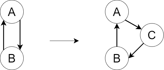
We perform the transformation above for all the reverse edges in the graph.

2.2. Residual Graph

The residual graph, R_G , of is defined in the following way: G_R = (G.V, E_R) , where $(u, v) \in E_R$ if C(u, v) - F(u,v ) > 0 in . Shortly, G_R consists of the same vertices as , and any edge $(u, v) \in G.E$ is present in E_R if (u, v) has the potential to conduct more flow. If for edge $(u, v) \in E$ , C(u, v) - F(u, v) = 0 , that means the edge’s capacity is fully used, and it can’t accept any more flow. Such an edge is absent in E_R .

Additionally, we include reverse edges in E_R . Reverse edges are absent in and may appear in E_R while running the Ford-Fulkerson method. If edge $(u, v) \in E$ currently conducts the flow of value F(u, v) , then we add edge (v, u) to E_R with residual capacity F(u, v) .

Finally, we define a positive function of residual capacities on the edges of E_R : $\textrm{C_R}: V \times V \rightarrow R$ . C_R is defined as:

$C_R(u, v) = C(u, v) - F(u, v), (u, v) \in E$ and
$C_R(v, u) = F(u, v), (u, v) \in E$ and

2.3. Augmenting Paths

An augmenting path is any path from $\boldsymbol{S}$ to $\boldsymbol{T}$ in $\boldsymbol{G_R}$ . They’re used by the algorithm to increase the flow from to gradually.

3. Edmonds-Karp Algorithm

3.1. Algorithm Demonstration

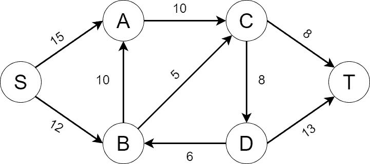
Assume we have a network graph shown below. The edge capacities are depicted as well:

network graph

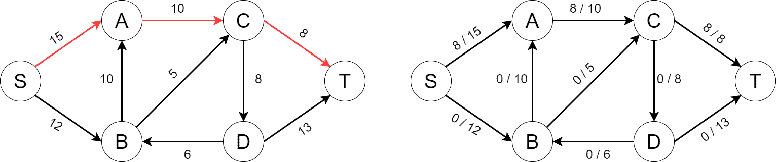
Let’s show how the Edmonds-Karp algorithm works by finding the maximum flow on the graph step by step. Initially, we build G_R , which fully matches as there’s no flow in yet. Below, we can see G_R on the left and on the right. For the edges of , we depict the current flow on them followed by their capacity:

ng state 1

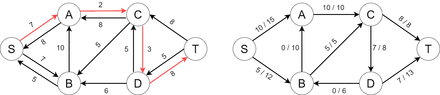
Next, we find the first shortest path from to using BFS. The path consists of three edges and is shown on G_R below. The flow increases by 8 along the augmenting path. We parallelly change the flow across the edges of as the algorithm progresses:

ng state 2

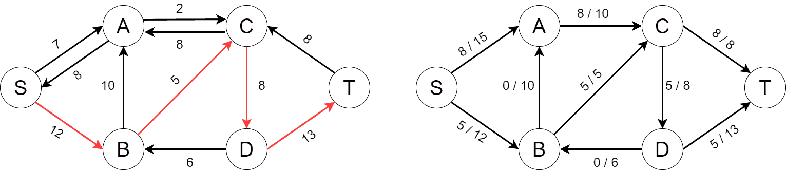
As the flow changes, new reverse edges may appear in G_R . Below, we can see new reverse edges, along with the second shortest path from to consisting of four edges. The flow increases by 5 this time:

ng state 3

Next, we find another augmenting path consisting of four edges. The path increases the flow by 2:

ng state 4

We’re in a situation now where there’re no augmenting paths left in G_R . It’s the indication that the algorithm has finished and we’ve found the maximum flow from to :

ng state 5

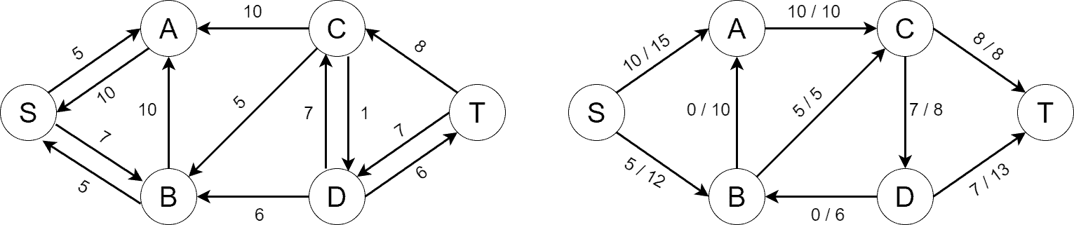
The maximum flow value may be fetched by either adding the flows on the outgoing edges of or by adding the flows on the incoming edge of . In either case, the maximum flow value is 15 for our example.

3.2. Algorithm Pseudocode

The pseudocode of the Edmonds-Karp algorithm is almost the same as the one for the Ford-Fulkerson method. The difference is that the Ford-Fulkerson method doesn’t specify how augmenting paths are found, while the Edmonds-Karp algorithm states they’re found using BFS. We can find the pseudocode of the Edmonds-Karp algorithm below:

algorithm EdmondsKarp(G, S, T):
    // INPUT
    //    G = the graph
    //    S = the source vertex
    //    T = the sink vertex
    // OUTPUT
    //    the maximum flow is found and returned

    // Build G_R
    Build G_R

    while there is an augmenting path p found by BFS(G_R):
        cmin <- infinity

        for (u, v) in p:
            if C_R(u, v) < cmin:
                cmin <- C_R(u, v)

        for (u, v) in p:
            if (u, v) in E:
                F(u, v) <- F(u, v) + cmin
            else:
                F(v, u) <- F(v, u) - cmin

            if (v, u) not in E_R:
                Add (v, u) to E_R
                C_R(v, u) <- 0

            C_R(u, v) <- C_R(u, v) - cmin
            C_R(v, u) <- C_R(v, u) + cmin

            if C_R(u, v) = 0:
                Remove (u, v) from E_R

    fmax <- 0

    for (u, T) in E:
        fmax <- fmax + F(u, T)

    return fmax

3.3. Algorithm Complexity

The drawback of the Ford-Fulkerson method is that it may run in exponential time. Its time complexity is $\boldsymbol{O(M * F_{max})}$ , where $\boldsymbol{F_{max}}$ is the value of the maximum flow. So, the method’s time complexity depends on the maximum flow value. It effectively means that we may have various performances by changing the capacity function on the same graph. Additionally, the Ford-Fulkerson method may never end if the capacities of the edges are irrational.

The Edmonds-Karp algorithm fixes the drawbacks as it runs in polynomial time: $\boldsymbol{O(N * M^2)}$ . The complexity follows from the observation that there can’t be more than $\boldsymbol{O(N * M)}$ flow augmentations, and each flow augmentation runs in $\boldsymbol{O(M)}$ .

4. Conclusion

In this tutorial, we’ve discussed the Edmonds-Karp algorithm for finding the maximum flow in network graphs. It’s a customization of the Ford-Fulkerson method where augmenting paths are found using BFS. The algorithm is polynomial.

Persistence

REST

Security