1. Introduction
Optical flow estimation is a fundamental technique used in computer vision to determine the motion of objects in consecutive images.
In this tutorial, we’ll explain the approach called coarse-to-fine flow estimation, used to compute the optical flow when large motion exists between images.
2. Fundamentals of Optical Flow
Optical flow is the motion of brightness patterns due to the relative motion between the observer and the scene. It is a fundamental concept in computer vision and has numerous applications, such as object tracking, video compression, and autonomous driving.
Optical flow is represented as a 2D vector field, where each vector corresponds to the displacement of a pixel. The motion field is computed using pixels of two consecutive video sequence frames.
There are two main types of optical flow methods: dense and sparse. Dense methods estimate the motion field for all pixels in the image, while sparse methods estimate the motion only for a subset of pixels.
Optical flow estimation is an ill-posed problem, meaning that infinitely many possible solutions can explain the observed motion. The optical flow constraint equation is the main formula for estimating the optical flow when the pixel displacement is small and the brightness constancy assumption is valid.
However, the simple linear optical flow constraint equation is no longer valid when a large motion exists between images. To address this challenge, a resolution pyramid concept is used to compute lower-resolution versions of the images, which reduces the magnitude of motion and makes the optical flow constraint equation valid again.
The coarse-to-fine approach involves starting with the lowest-resolution images and applying an optical flow algorithm to estimate the flow, which is then used to warp the image in the next higher resolution. This process is repeated until the highest resolution images are reached, resulting in the final optical flow estimation.
3. Resolution Pyramid
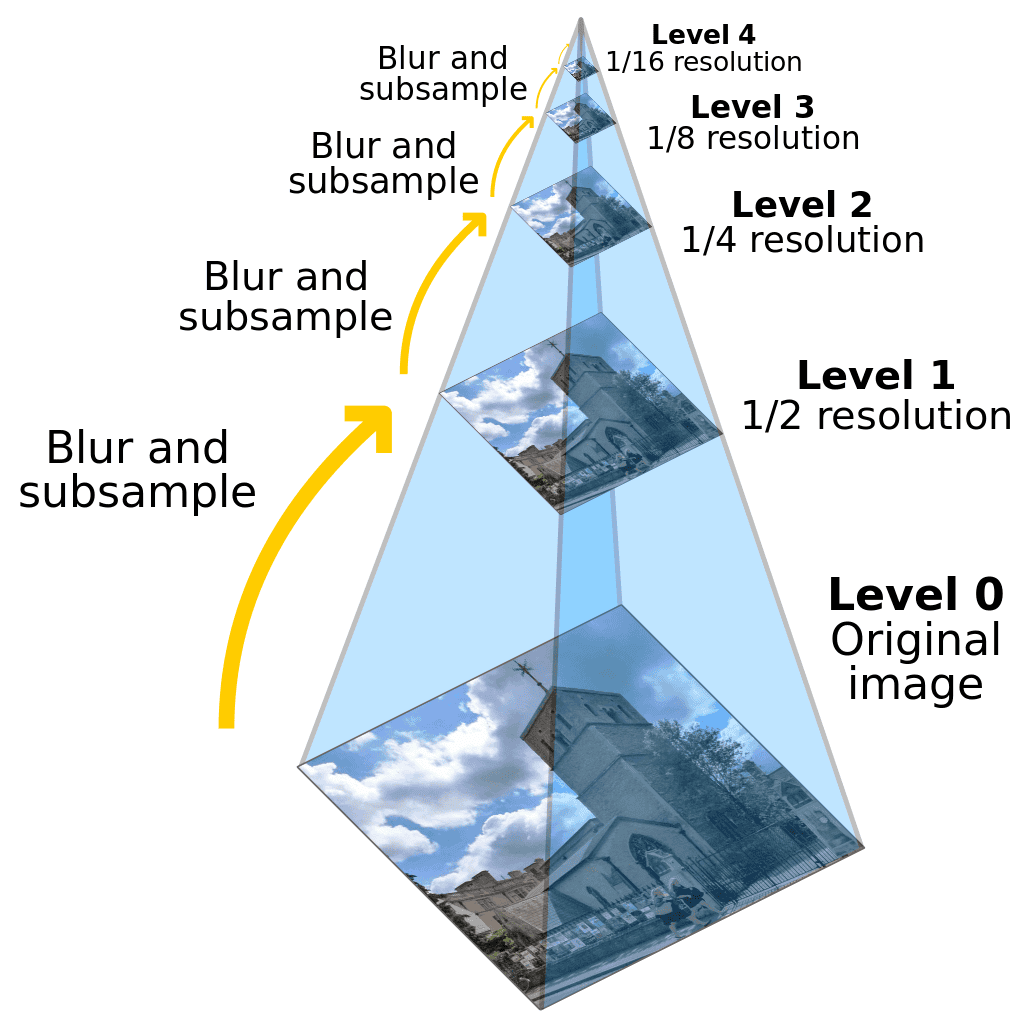
The resolution pyramid concept involves computing a series of images, each with successively lower resolution, by applying iterative downsampling techniques. Reducing the resolution reduces the motion of a particular scene point, which makes the optical flow constraint equation valid again.
The following figure represents the computation of the resolution pyramid. The image in the upper level is obtained by burring and downsampling the image at the previous level.
The algorithm for going from coarse to fine estimation of optical flow involves starting with the lowest resolution images and applying the optical flow algorithm. The optical flow is then used to warp the image in the next higher resolution. This process is repeated until the highest resolution images are reached, and the final flow is obtained.
This method works well because it propagates information from lower resolutions to higher resolutions while ensuring that the optical flow constraint equation remains valid. The resulting optical flow vectors reveal the speed and direction of motion for each point in the image.
4. Coarse-To-Fine Optical Flow Estimation Algorithm
The Coarse-to-Fine Optical Flow Estimation Algorithm allows us to estimate the optical flow in images with large motion between consecutive images. The algorithm uses a resolution pyramid to compute lower-resolution versions of the images, which reduces the magnitude of the motion of a particular scene point.
The algorithm involves the following steps:
- Compute lower-resolution versions of the two consecutive images (acquired at time
 and
and  ) by taking each 2×2 window in one of the images, finding the average of those values, and using that value in the new low-resolution image
 - Start with the lowest resolution images and apply the optical flow algorithm, such as Lucas-Kanade’s algorithm, to compute the optical flow
- Use the optical flow resulting from the previous step to warp the image at in the next higher resolution
- Compute the optical flow between the warped image and image at . Finally, add the result to the previous optical flow estimate
- Keep repeating steps 3 and 4 until arriving at the highest-resolution images, which gives the final flow
The following figure is a schematic representation of the algorithm.
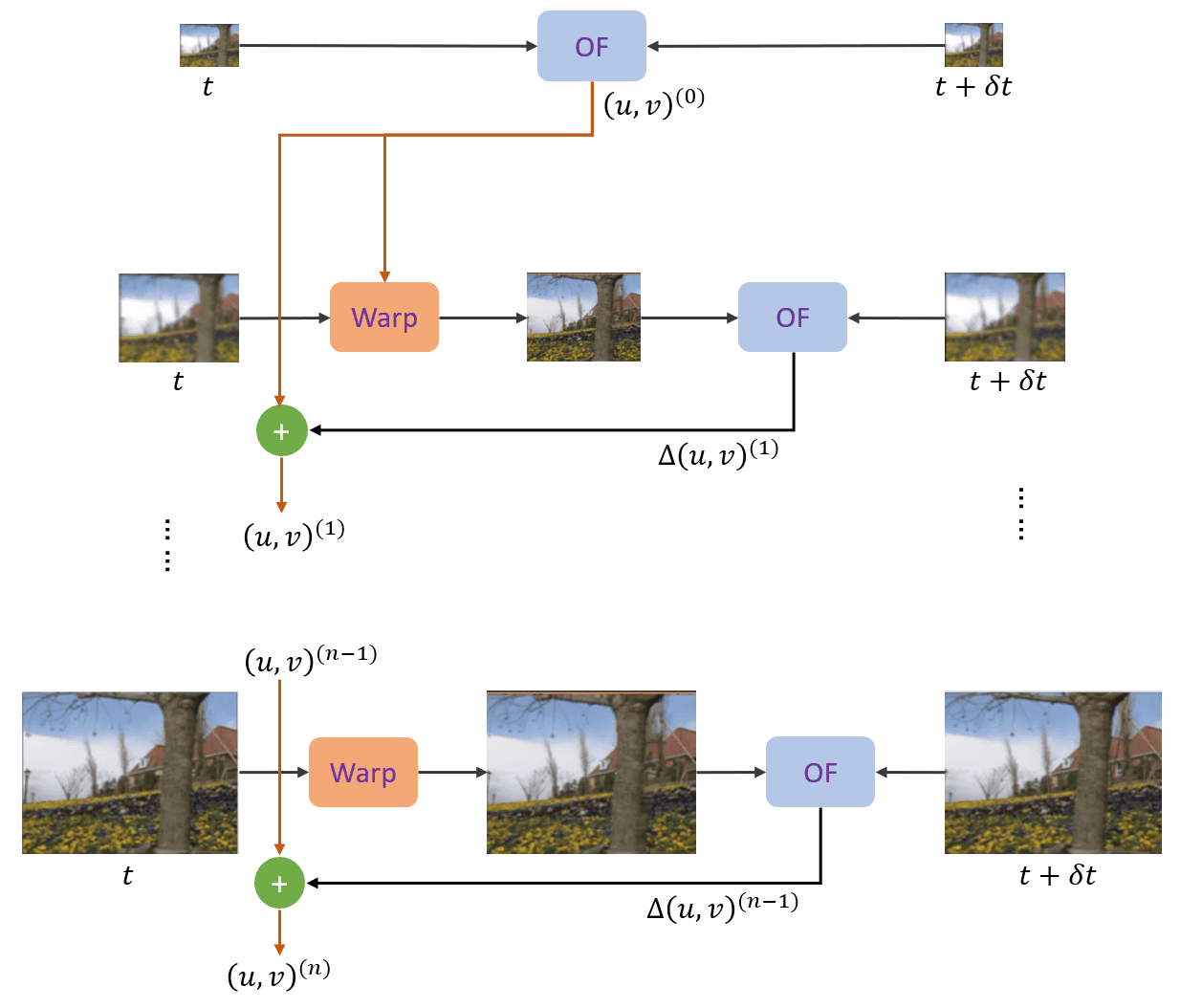
The method works well because it propagates information from lower to higher resolutions while ensuring the optical flow constraint equation remains valid. By using a pyramidal representation and refining the flow estimate at each level, this approach can produce high-quality flow fields that are useful in a wide range of computer vision applications.
An alternative approach to computing optical flow is template matching, but it is less advantageous than the described approach exploiting the resolution pyramid.
5. Template Matching Approach
This approach involves using a small window in the image at time as a template and searching for the best match in the image at time . The search space needs to be large enough to account for the magnitude of motion, which is not known beforehand. The difference between the locations of the two windows is the optical flow vector.
However, this approach can be slow, especially if a large search space is used. Additionally, mismatches can occur, as the method does not use local image derivatives.
6. Conclusion
In this article, we reviewed the concept of optical flow and the methods to compute it. In particular, we explained the coarse-to-fine flow estimation that effectively addresses the challenge of computing optical flow in the presence of large motion. By leveraging a resolution pyramid, this method ensures the validity of the optical flow constraint equation, resulting in accurate motion estimation. Finally, we described an alternative approach based on template matching.