Probability Calibration of Binary Classifiers

1. Introduction

In this tutorial, we’ll explain the calibration of probabilistic binary classifiers.

We’ll define calibrated classifiers, explain how to check if a classifier is such, and how to obtain calibrated classifiers during training or by postprocessing the existing ones.

2. Probabilities and Classification

Some binary classifiers estimate the probability p(x) that the input object is positive. We call them probabilistic binary classifiers and classify as positive if $p(x) \geq 0.5$ and as negative if p(x) < 0.5 .

If p(x) does represent a probability that is positive, we’ll expect to have $\boldsymbol{100t\%}$ positive objects among those for which the estimated probability $\boldsymbol{p(x)}$ is equal to $\boldsymbol{t \in [0, 1]}$ . Otherwise, the values p(x) don’t behave as probabilities and aren’t informative.

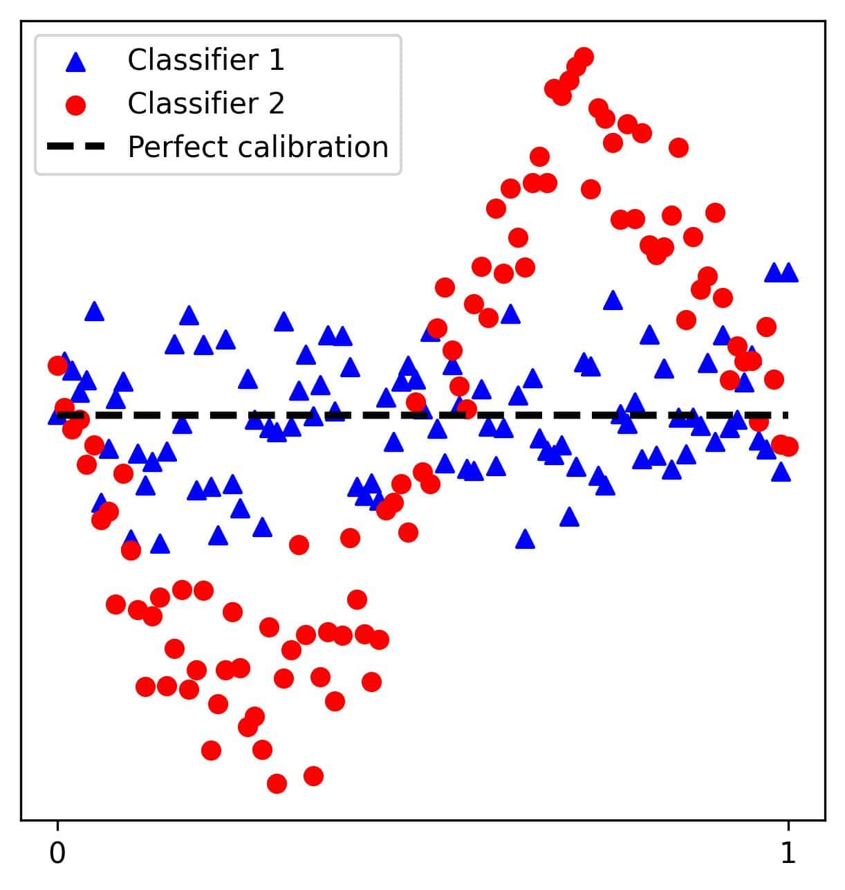
Let’s consider two classifiers. Both estimate the probability of the input object being positive:

They have the same accuracy, but their probability estimates aren’t equally reliable. Why is this important? If a classifier tells us that there’s a 30% chance of rain, we’d like it to be right 30% of the time.

This property should hold for any probability estimate $t \in [0\%, 100\%]$ . Such classifiers are more reliable as we can distinguish between likely, unlikely, and uncertain events. For example, we won’t take an umbrella if the probability of rain is 5%, but we will if it’s 45%, 55%, or higher.

The classifiers whose probability estimates are reliable in this sense are called perfectly or well-calibrated.

3. Calibration

Mathematically, we define well-calibrated classifiers as follows. Let denote the ground-truth label of a random object (0 or 1), and let denote the probability. Then, a classifier with the probability estimates $p(\cdot)$ is well-calibrated if:

$[(\forall t \in [0, 1]) P\left(Y=1 \mid p(X) = t \right) = t]$

Let $\pi_t = P\left(Y=1 \mid p(X) = t \right)$ . Geometrically, the mapping $t \mapsto \pi_t$ of well-calibrated classifiers corresponds to the identity function over [0, 1] .

If the graph of $t \mapsto p_t$ is under the identity line, the values p(x) underestimate the probabilities $\pi_{p(x)}$ . Conversely, our classifier’s output score p(x) overestimates $\pi_{p(x)}$ if the graph is above the identity line.

The probabilities $\boldsymbol{\pi_{p(x)}}$ should be understood in the frequentist sense. So, for a well-calibrated classifier, p(x)=t doesn’t mean that the probability that the specific object is positive equals . Instead, if we classified an infinite number of objects using this classifier, 100t% of objects that got the score p(x)=t would be positive.

4. How to Check for Calibration?

We can check whether a classifier is well-calibrated using calibration metrics and diagnostic plots.

4.1. Miscalibration Score

Let’s assume that the output probability p(x) can take a finite number of values between 0 and 1. Let that set be $\mathcal{T}$ and let w_t be the probability that p(X)=t . We can define the miscalibration score as the expected squared deviation of the output probability estimates from true (frequentist) probabilities:

$[C = \sum_{t \in \mathcal{T}} w_t(p_t - t)^2]$

Let’s introduce the penalty for estimates close to 1/2:

$[R = \sum_{t \in \mathcal{T}}w_t \pi_t (1-\pi_t)]$

The sum of and is known as the Brier score . For a given test set $\{(x_i, y_i)\}_{i=1}^{n}$ , it can be calculated as follows:

$[B = C + R = \frac{1}{n}\sum_{i=1}^{n}(p(x_n) - y_n)^2]$

The Brier and miscalibration scores of 0 correspond to a perfectly calibrated probabilistic classifier.

4.2. Calibration by Overlapping Bins

Since the actual probabilities are unknown, we can’t directly compare the calibrated probabilities with the true ones on a per-instance basis. However, we can split the data into several bins and compare the average calibrated probability with the fraction of positive examples in each bin. The problem with this approach is that if we use too few or too many disjunctive bins, the bin averages will not be good estimates of the actual means.

Calibration by overlapping bins (COB) addresses the issue using overlapping bins of size and is calculated as follows. First, the objects are sorted by their calibrated probability and indexed from 1 to . So, we have the probability array $p_1 \leq p_2 \leq \ldots \leq p_n$ .

Then, we group the objects with indices 1 to in the first bin, 2 to s + 1 in the second, and so on. Let n_j^+ be the number of positive objects in the -th bin. We compute COB as the mean absolute difference between the average probabilities and fractions of positive examples in all bins:

$[COB = \frac{1}{n-s} \sum_{j=1}^{n-s} \left| \left(\frac{1}{s} \sum_{i=j}^{j+s-1}p_i\right) - \frac{n_j^+}{s}\right|]$

The more calibrated a classifier is, the closer COB is to zero.

To make COB independent of , we can use $s=\alpha n$ as the bin size, where $\alpha$ is a positive float lower than 1. The chosen size shouldn’t result in too narrow or too broad bins.

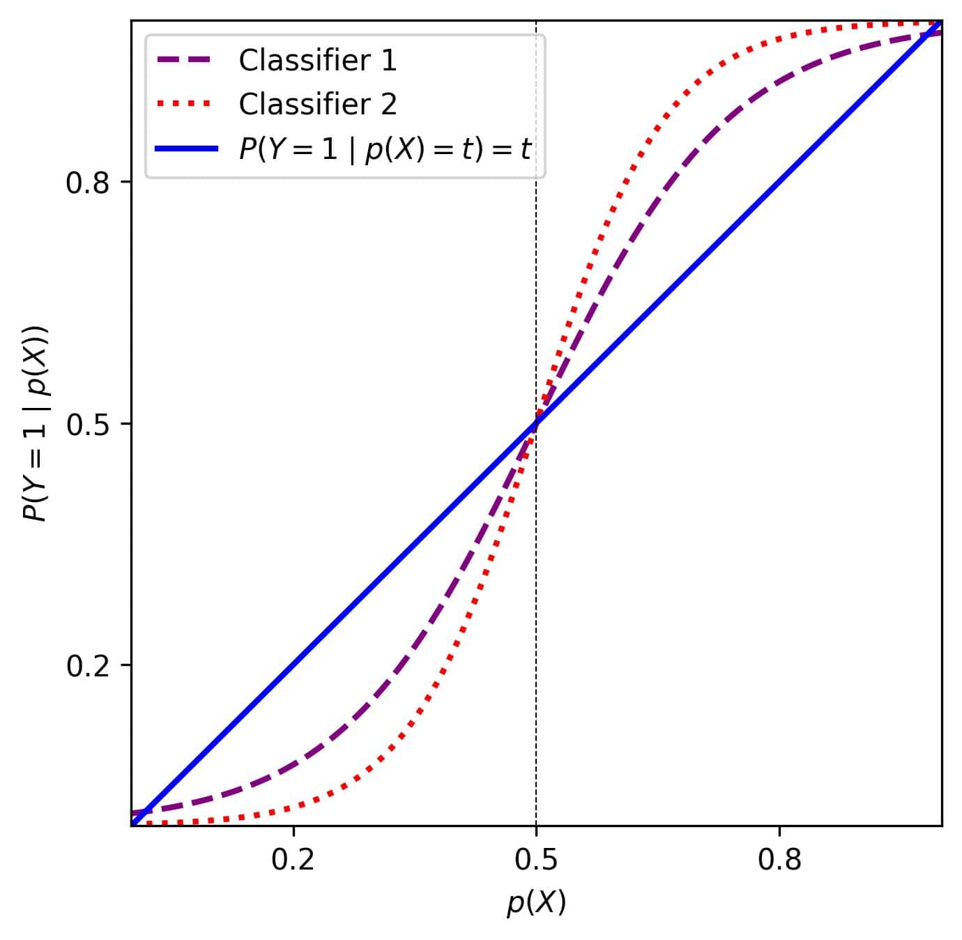
4.3. Reliability Diagrams

A reliability diagram visualizes the relationship between predicted and actual probabilities.

To make it, we first discretize data into several same-size bins. Then, we plot the actual frequency of positive objects in a bin against the
expected proportion of positive examples. The expected proportion in a bin is the mean probability of objects it contains.

More formally, the th bin contains the objects $x_{(j-1)s+1}$ , $x_{(j-1)s+2}$ , …, $x_{js}$ . Let n_j^+ be the number of positive objects in the th bin. A reliability diagram visualizes the mapping:

$[\left(\frac{1}{s}\sum_{i=(j-1)s+1}^{js}p_i \right) \quad \mapsto \quad \frac{n_j^+}{s}]$

If the probabilities are well-calibrated, the resulting line should resemble the 45-degree line:

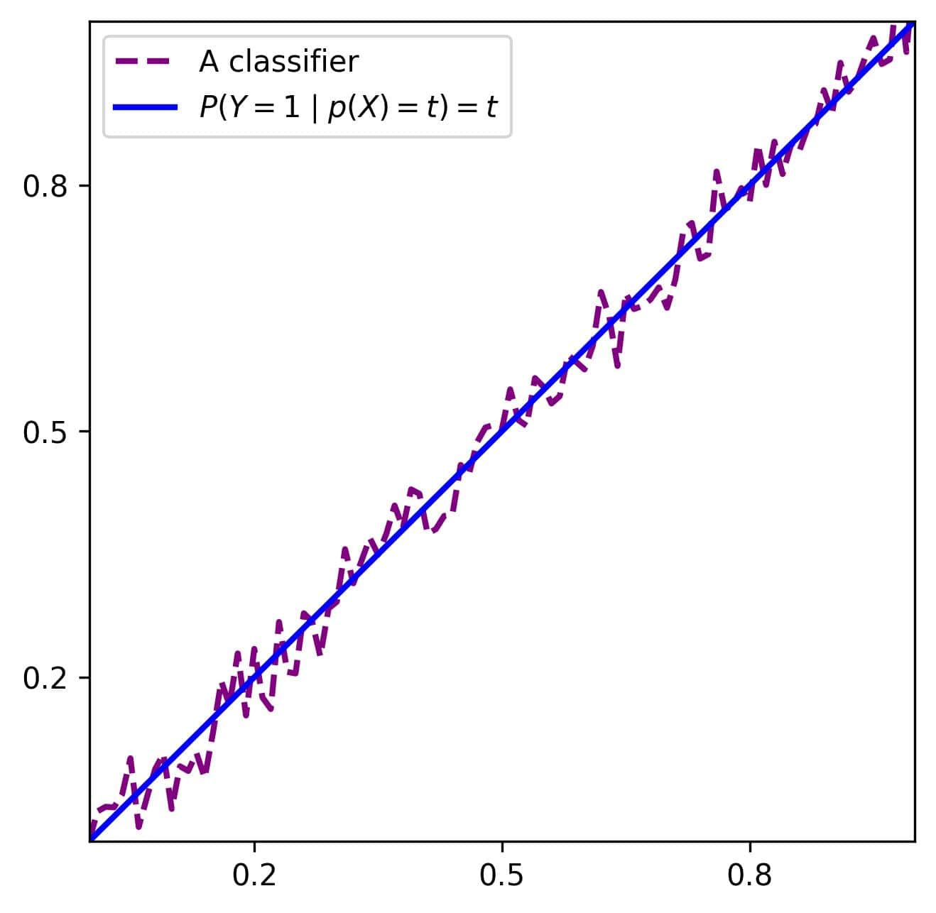
4.4. Deviation Plots

We also sort and discretize probabilities into even-sized bins to make this plot. However, instead of the actual frequencies $\boldsymbol{n_j^+/s}$ on the $\boldsymbol{y}$ -axis, we plot the deviations, so the mapping is:

$[\left(\frac{1}{s}\sum_{i=(j-1)s+1}^{js}p_i \right) \quad \mapsto \quad \left(\frac{1}{s}\sum_{i=(j-1)s+1}^{js}p_i\right) - \frac{n_j^+}{s}]$

This scatter plot of deviations can reveal systematic errors in the probabilistic classifiers. If the deviations don’t appear to be scattered randomly around zero, that indicates that the model isn’t calibrated well:

5. How to Calibrate a Classifier?

There are two main approaches: during training or postprocessing.

5.1. Training vs. Postprocessing

We can try to train an already calibrated classifier. To do that, we can minimize the Brier score or add COB or the miscalibration score as a penalty to the cost function of our choice.

However, we don’t always have the resources to train a classifier from scratch. Additionally, introducing penalties might slow training down. In such cases, we can train our classifier as usual and post-process it after training to calibrate its probabilities. An advantage of this approach is that we can apply it to existing classifiers.

We’ll cover two postprocessing methods: Platt scaling and isotonic regression.

5.2. Platt Scaling

Let $f(\cdot)$ be the scoring function of the classifier we want to calibrate. The scores can be probabilities, but that’s not necessary.

Platt scaling learns a mapping from -scores to the probabilities $p(x)=P(Y = 1 \mid f(x))$ :

$[p(x) = \frac{1}{1+\exp{(A f(x) + B)}}]$

where the coefficients and are obtained by minimizing the cost:

$[-\sum_{i=1}^{n}\left( y_i \log(p(x_i)) + (1 - y_i) \log(1 - p(x_i)) \right)]$

using set $\{(x_i, y_i)\}_{i=1}^{n}$ held out for calibration.

Platt scaling assumes that the class-conditional distributions of the $\boldsymbol{f}$ scores are exponential, so this technique is an example of a parametric calibration method.

These methods assume the analytical form of the mapping to the probabilities, which we derive from the exponential distributions in the case of Platt scaling. If our data violate the assumption, the calibrated probabilities may be unreliable.

5.3. Isotonic Regression

Isotonic regression is a non-parametric calibration technique, as it doesn’t assume the analytical form of the mapping (or class-conditional densities).

In isotonic regression, we sort the held-out objects objects $x_1, x_2, \ldots, x_n$ by their scores to get $x_{(1)}, x_{(2)}, \ldots, x_{(n)}$ such that $f(x_{(i)}) \leq f(x_{(i+1)})$ for all $i=1,2,\ldots, n-1$ . Our goal is to find the corresponding probabilities $p_{(1)}, p_{(2)}, \ldots, p_{(n)}$ that minimize the Brier Score and are non-decreasing:

$[\min_{p_{(1)}, \ldots, p_{(n)}} \frac{1}{n} \sum_{i=1}^{n}(p_{(i)}-y_{(i)})^2 \qquad \text{s.t. } p_{(1)} \leq p_{(2)} \leq \ldots \leq p_{(n)} \text{ and } (\forall i = 1, 2, \ldots, n)(p_{(i)} \in [0, 1])]$

where $y_{(i)}$ is the true label of $x_{(i)}$ .

After finding the $p_{(i)}$ , we can determine p(x) of a new object as follows:

compute its -score
find and such that $f(x_{(i)}) \leq f(x) < f(x_{(i+1)})$
return $p(x)=\frac{1}{2}(p_{(i)} + p_{(i+1)})$

If $f(x) < f(x_{(1)})$ , we can output $p(x)=p(x_{(1)}) - \Delta$ , for some small value $\Delta$ . Similarly, if $f(x) \geq f(x_{(n)})$ , our output can be $p(x_{(n)}) + \Delta$ .

6. Choosing the Calibration Method

There are other calibration methods, such as beta calibration, histogram binning, and adaptive calibration of probabilities. Which one we should choose depends on the classifier model and data.

As a rule of thumb, we can use a parametric method if its assumptions are met. Otherwise, we can go for a non-parametric method. However, if we have enough data to test calibration, we can try several methods and use the one that returns the best-calibrated probabilities.

7. Conclusion

In this article, we explained calibration, how to check if a classifier is calibrated, and how to calibrate its output to get reliable probabilities.

Uncalibrated classifiers might have acceptable classification accuracy, but calibrated probabilities are preferred because their probability estimates are more reliable.

Persistence

REST

Security