1. 简介
在本文中,我们将深入理解 粒子群优化算法(Particle Swarm Optimization, PSO) 的工作原理。首先介绍其起源与灵感来源,然后详细讲解算法的数学模型与执行步骤,并配以流程图。最后,我们会列举一些实际应用场景,并通过一个神经网络训练的案例来展示其应用方式。
2. 起源与灵感
自然界中生物群体的行为启发了大量人工智能算法的发展。这些算法大致可分为两类:
- 个体行为启发:如神经网络、遗传算法等,模拟细胞或神经元的行为。
- 群体行为启发:如蚁群、蜂群、鸟群等,统称为 群体智能(Swarm Intelligence)。
PSO 属于第二类,是一种 基于群体智能的元启发式优化算法,由 James Kennedy 和 Russell Eberhart 于 1995 年提出。
2.1 关键术语解释
- 优化问题:从多个可行解中寻找最优解。
- 元启发式算法:不依赖具体问题、适用于多种优化问题的通用策略。
- 群体智能:通过多个个体的局部交互与协作,形成全局智能行为。
常见的群体智能算法包括蚁群算法、灰狼优化、鲸鱼优化、蚁狮优化等。
3. 粒子群优化算法详解
PSO 是一种基于种群的优化算法,通过模拟鸟群在空间中搜索食物的行为来寻找最优解。
3.1 工作原理
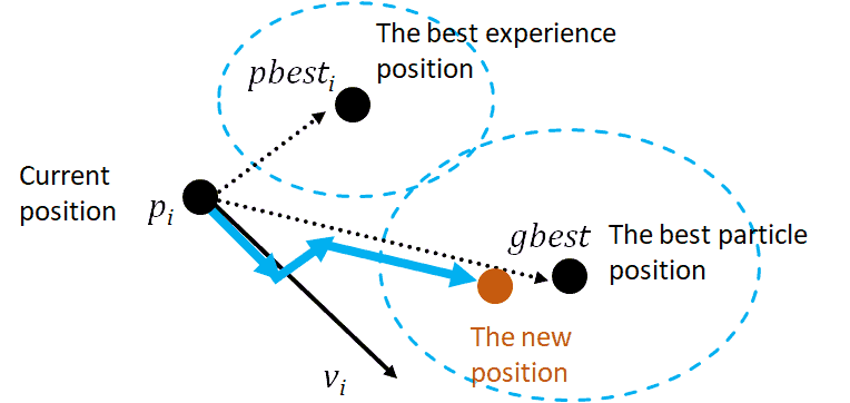
PSO 使用一组粒子(particles)组成“群体”,每个粒子代表一个候选解。所有粒子在解空间中飞行,根据以下两个经验动态调整自己的速度和位置:
✅ 自身历史最优解(pbest)
✅ 全局最优解(gbest)
每个粒子通过不断更新自己的位置和速度,逐步逼近最优解。
3.2 核心参数
以下是 PSO 中常用参数:
S(n) = {s₁, s₂, ..., sₙ}:由 n 个粒子组成的群体sᵢ:第 i 个粒子pᵢ:粒子的位置vᵢ:粒子的速度pbestᵢ:粒子自身历史最优解gbest:整个群体的历史最优解f:适应度函数c₁, c₂:认知和社会加速常数r₁, r₂:[0,1] 区间内的随机数t:当前迭代次数
3.3 数学模型
PSO 主要依赖两个公式:
✅ 速度更新公式:
$$ v_i^{t+1} = w \cdot v_i^t + c_1 \cdot r_1 \cdot (pbest_i - p_i^t) + c_2 \cdot r_2 \cdot (gbest - p_i^t) $$
✅ 位置更新公式:
$$ p_i^{t+1} = p_i^t + v_i^{t+1} $$
其中:
w是惯性权重,控制粒子的探索与开发能力c₁表示个体信任度c₂表示群体信任度r₁和r₂增加随机性,避免陷入局部最优
粒子的更新过程如下图所示:
3.4 执行步骤与流程图
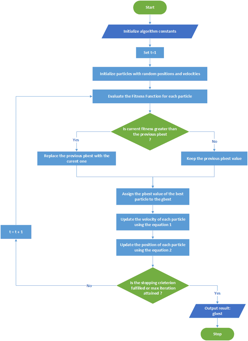
PSO 的执行流程如下:
- 初始化参数(种群大小、速度、位置等)
- 评估每个粒子的适应度
- 更新个体最优解(pbest)和全局最优解(gbest)
- 按照公式更新速度和位置
- 判断是否满足终止条件(如最大迭代次数),若否则返回步骤 2
流程图如下:
4. PSO 应用场景
PSO 算法因其简单、高效、无需导数等优点,广泛应用于多个领域,包括:
- 神经网络训练(如识别帕金森病、图像识别)
- 电力系统优化
- 结构设计优化(形状、尺寸、拓扑结构)
- 生物力学系统建模与识别
5. 使用 PSO 训练神经网络的实践案例
我们以 Iris 花朵分类问题 为例,演示如何使用 PSO 来训练一个简单的神经网络。
5.1 神经网络实现
我们构建一个两层网络:一个隐藏层 + 一个输出层。输入层接收 4 个特征(花萼长宽、花瓣长宽),输出层输出 3 个类别的概率。
- 隐藏层使用 Sigmoid 激活函数
- 输出层也使用 Sigmoid,最后通过 Softmax 转换为概率分布
import numpy as np
from sklearn.datasets import load_iris
from sklearn.model_selection import train_test_split
from sklearn.preprocessing import StandardScaler, OneHotEncoder
from sklearn.metrics import accuracy_score, confusion_matrix

def sigmoid(x):
    return 1 / (1 + np.exp(-x))

def softmax(x):
    e_x = np.exp(x - np.max(x))
    return e_x / e_x.sum(axis=1, keepdims=True)

def train_network_forward_propagation(weights, hidden_layer_size, X_train_data, y_train_data):
    # 权重拆分
    hidden_layer_weights = weights[:4*hidden_layer_size].reshape(4, hidden_layer_size)
    output_layer_weights = weights[4*hidden_layer_size:].reshape(hidden_layer_size, 3)

    # 前向传播
    hidden_layer_input = np.dot(X_train_data, hidden_layer_weights)
    hidden_layer_output = sigmoid(hidden_layer_input)
    output_layer_input = np.dot(hidden_layer_output, output_layer_weights)
    output_layer_output = sigmoid(output_layer_input)

    # 损失计算(均方误差)
    loss = np.mean(np.square(y_train_data - output_layer_output))
    return loss

def evaluate_network(weights, hidden_layer_size, X_test, y_test):
    # 权重拆分
    hidden_layer_weights = weights[:4*hidden_layer_size].reshape(4, hidden_layer_size)
    output_layer_weights = weights[4*hidden_layer_size:].reshape(hidden_layer_size, 3)

    # 前向传播
    hidden_layer_input = np.dot(X_test, hidden_layer_weights)
    hidden_layer_output = sigmoid(hidden_layer_input)
    output_layer_input = np.dot(hidden_layer_output, output_layer_weights)
    output_layer_output = sigmoid(output_layer_input)

    # Softmax 转换为概率
    predictions = softmax(output_layer_output)
    predicted_classes = np.argmax(predictions, axis=1)
    true_classes = np.argmax(y_test, axis=1)

    # 准确率与混淆矩阵
    accuracy = accuracy_score(true_classes, predicted_classes)
    conf_matrix = confusion_matrix(true_classes, predicted_classes)

    return accuracy, conf_matrix
5.2 PSO 算法实现
我们使用 PSO 对神经网络进行训练,每个粒子代表一组网络权重。目标函数为前向传播计算的损失值。
def pso_iris(num_particles, num_iterations, hidden_layer_size, X_train_data, y_train_data):
    num_dimensions = 4 * hidden_layer_size + hidden_layer_size * 3
    positions = np.random.rand(num_particles, num_dimensions) - 0.5  # 初始化位置
    velocities = np.zeros_like(positions)  # 初始化速度
    pbest_positions = np.copy(positions)
    pbest_scores = np.array([train_network_forward_propagation(p, hidden_layer_size, X_train_data, y_train_data) for p in positions])
    gbest_position = pbest_positions[np.argmin(pbest_scores)]
    gbest_score = np.min(pbest_scores)

    # PSO 迭代
    w = 0.5  # 惯性权重
    c1 = 2   # 个体信任度
    c2 = 2   # 群体信任度

    for i in range(num_iterations):
        for j in range(num_particles):
            r1, r2 = np.random.rand(2)
            velocities[j] = w * velocities[j] + c1 * r1 * (pbest_positions[j] - positions[j]) + c2 * r2 * (gbest_position - positions[j])
            positions[j] += velocities[j]

            current_score = train_network_forward_propagation(positions[j], hidden_layer_size, X_train_data, y_train_data)
            if current_score < pbest_scores[j]:
                pbest_scores[j] = current_score
                pbest_positions[j] = positions[j]

        # 更新全局最优
        current_gbest_score = np.min([train_network_forward_propagation(p, hidden_layer_size, X_train_data, y_train_data) for p in positions])
        if current_gbest_score < gbest_score:
            gbest_score = current_gbest_score
            gbest_position = positions[np.argmin([train_network_forward_propagation(p, hidden_layer_size, X_train_data, y_train_data) for p in positions])]

        print(f"Iteration {i+1} - Best Loss: {gbest_score}")

    print("Optimal Weights Found by PSO:", gbest_position)
    return gbest_position
5.3 实验运行
加载数据集并进行预处理后,调用 PSO 函数进行训练,并评估模型性能。
# 加载数据集
iris = load_iris()
X, y = iris.data, iris.target
encoder = OneHotEncoder()
y_onehot = encoder.fit_transform(y.reshape(-1, 1))
X_train, X_test, y_train, y_test = train_test_split(X, y_onehot, test_size=0.2, random_state=42)

# 数据标准化
scaler = StandardScaler()
X_train_scaled = scaler.fit_transform(X_train)
X_test_scaled = scaler.transform(X_test)

# PSO 训练
hidden_layer_size = 6
iris_classifier = pso_iris(30, 50, hidden_layer_size, X_test_scaled, y_test)

# 模型评估
accuracy, conf_matrix = evaluate_network(iris_classifier, hidden_layer_size, X_test_scaled, y_test)
print("Accuracy:", accuracy)
print("Confusion Matrix:\n", conf_matrix)
实验结果显示,在使用 6 个隐藏层神经元、30 个粒子、50 次迭代后,模型准确率达到 **90%**,仅误分类 3 个样本。
6. 总结
本文详细介绍了 粒子群优化算法(PSO) 的原理、数学模型与实际应用。我们通过一个神经网络训练的实战案例,展示了 PSO 在优化问题中的强大能力。
PSO 以其简单高效、参数少、无需导数等优点,成为解决多领域优化问题的重要工具。无论是工程优化、机器学习、还是系统建模,PSO 都有广泛的应用前景。