1. 概述
在本教程中,我们将探讨如何查找具有特定和 K 的子数组个数。
我们会先定义问题并举例说明。然后介绍两种不同的解法:暴力枚举法 和 前缀和优化法,并分析它们的实现方式和时间复杂度。最后总结两者的优劣。
2. 问题定义
给定一个数组 A,我们需要统计其中所有连续子数组的和等于给定值 K 的个数。
✅ 子数组(Subarray) 是指数组中一段连续的子序列。
示例
给定数组 A = [1, 3, 0, 5, -2],目标和 K = 3,那么满足条件的子数组如下(图中红色部分):
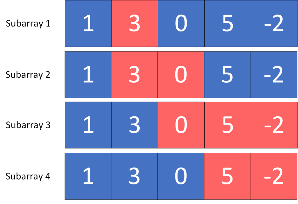
共有 4 个子数组满足条件,分别是:
- [1, 3]
- [3]
- [0, 3]
- [5, -2]
3. 暴力枚举法
3.1 思路说明
暴力解法的核心是:枚举所有可能的子数组,计算它们的和,并统计等于 K 的数量。
具体做法是:
- 固定子数组的起始位置
start - 枚举所有可能的结束位置
end - 在每次扩展
end时累加元素值,计算当前子数组的和 - 若当前和等于
K,则计数器加一
这种方式虽然直观,但效率较低。
3.2 实现代码
public int countSubarrays(int[] A, int K) {
    int answer = 0;
    int n = A.length;

    for (int start = 0; start < n; start++) {
        int sum = 0;
        for (int end = start; end < n; end++) {
            sum += A[end];
            if (sum == K) {
                answer++;
            }
        }
    }

    return answer;
}
3.3 时间复杂度分析
- 外层循环枚举所有起始位置:
O(N) - 内层循环枚举所有结束位置:
O(N) - 总体复杂度为
O(N²)
对于大数组来说性能较差,存在优化空间。
4. 前缀和优化法(Prefix Sum)
4.1 思路说明
我们利用前缀和的概念来优化查找效率。
✅ 前缀和(Prefix Sum) 是指从数组起始位置到当前位置的元素和。
假设我们有一个前缀和数组 prefixSum,其中 prefixSum[i] 表示从 A[0] 到 A[i-1] 的和。
那么任意子数组 A[i..j] 的和可以表示为:
sum(A[i..j]) = prefixSum[j+1] - prefixSum[i]
我们想要找的是满足:
prefixSum[j+1] - prefixSum[i] = K
即:
prefixSum[i] = prefixSum[j+1] - K
因此,我们可以在遍历过程中维护一个哈希表,记录每个前缀和出现的次数。这样可以在 O(1) 时间内快速查找符合条件的前缀和个数。
4.2 实现代码
import java.util.HashMap;

public int countSubarrays(int[] A, int K) {
    HashMap<Integer, Integer> count = new HashMap<>();
    int[] prefixSum = new int[A.length + 1];

    // 计算前缀和
    for (int i = 0; i < A.length; i++) {
        prefixSum[i + 1] = prefixSum[i] + A[i];
    }

    int answer = 0;
    count.put(0, 1); // 初始前缀和为 0 出现一次

    for (int sum : prefixSum) {
        answer += count.getOrDefault(sum - K, 0);
        count.put(sum, count.getOrDefault(sum, 0) + 1);
    }

    return answer;
}
4.3 时间复杂度分析
- 前缀和数组构造:
O(N) - 遍历前缀和数组并维护哈希表:
O(N) - 总体复杂度为
O(N)
这是目前最优的解法,适用于大数组场景。
5. 总结
我们介绍了两种查找满足特定和的子数组个数的方法:
| 方法 | 时间复杂度 | 是否推荐 | 说明 |
|---|---|---|---|
| 暴力枚举法 | O(N²) |
❌ | 实现简单但效率低 |
| 前缀和优化法 | O(N) |
✅ | 利用哈希表优化查找效率,推荐使用 |
⚠️ 踩坑提醒:暴力法在 LeetCode 等平台容易超时,建议优先使用前缀和优化法。
如果你对前缀和技巧不熟悉,建议多练习类似题型,如:
- LeetCode 560. Subarray Sum Equals K
- LeetCode 974. Subarray Sums Divisible by K
- LeetCode 525. Contiguous Array
这些题目都可以通过类似思路解决。