Ternary Search Tree 数据结构详解

1. 简介

在本教程中，我们将介绍 Ternary Search Tree（TST，三叉搜索树）这一数据结构。 它是一种非常有趣且高效的字符串查找结构，特别适用于需要频繁进行字符串检索的场景。

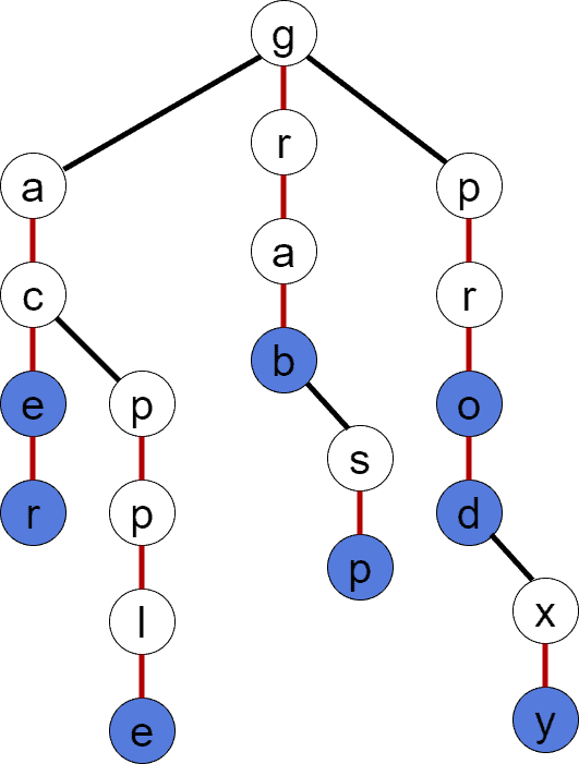
我们假设有一组字符串：

$$ S = {"ace", "acer", "apple", "grab", "grasp", "pro", "prod", "proxy"} $$

为简化讨论，我们假设这些字符串是按字典序排列的，并且每个字符串都按 1-indexed 方式处理字符。

为了便于后续分析复杂度，我们定义几个变量：

N：集合 S 中字符串的总数
M：S 中最长字符串的长度
A：构成字符串的字符集大小

这些变量将在后续章节中频繁使用。

2. TST 概述

TST 是一种高效的字符串查找数据结构，结合了二叉搜索树（BST）的空间效率和 Trie 的查找速度优势。

与 Trie 类似，TST 也是通过拆分字符串字符来构建树结构。但不同的是，每个节点最多有三个子节点，分别代表：

leftChild：值小于当前节点的子节点
middleChild：值等于当前节点的子节点，表示字符串中的下一个字符
rightChild：值大于当前节点的子节点

每个节点还包含：

value：当前字符
isTerminal：标记该节点是否是某个字符串的结尾

如下图所示是一个基于集合 S 构建的 TST 示例，蓝色节点为终止节点，红色边表示 middleChild：

tst

TST 的查找效率与树的深度密切相关。在理想平衡状态下，其查找复杂度为：

$$ O(M \cdot \log A) $$

空间复杂度方面，最坏情况下（无前缀共享）为：

$$ O(N \cdot M) $$

3. TST 操作详解

3.1 插入操作

插入操作的核心逻辑包括：

创建新节点
初始化子节点
设置终止标记

我们先定义一个辅助函数用于创建节点：

algorithm CREATE_NODE(val):
    node <- new TSTNode
    node.value <- val
    node.leftChild <- NULL
    node.middleChild <- NULL
    node.rightChild <- NULL
    node.isTerminal <- FALSE
    return node

然后是递归插入的实现：

algorithm INSERT(node, str, pos):
    if pos = str.length + 1:
        return node

    if node = NULL:
        node <- CREATE-NODE(str[pos])

    if str[pos] < node.value:
        node.leftChild <- INSERT(node.leftChild, str, pos)
    else if str[pos] > node.value:
        node.rightChild <- INSERT(node.rightChild, str, pos)
    else:
        if pos = str.length:
            node.isTerminal <- TRUE
        else:
            node.middleChild <- INSERT(node.middleChild, str, pos + 1)

    return node

✅ 关键点： 插入时如果当前字符匹配，则继续插入下一个字符；否则根据大小关系插入左右子树。

3.2 构建 TST

TST 的构建本质上就是多次插入操作。构建方式可分为两种：

离线模式（offline）：已知所有字符串，建议随机插入或按中位字符串递归插入
在线模式（online）：动态插入，建议使用平衡策略

以下是一个离线模式构建的伪代码：

algorithm TST_BUILD(S):
    rootNode <- NULL
    Shuffle S
    for s in S:
        rootNode <- INSERT(rootNode, s, 1)
    return rootNode

⚠️ 注意： 如果字符串是按字典序插入的，TST 可能退化为链表，性能下降明显。

3.3 查找操作

查找操作也是递归实现的，核心逻辑如下：

algorithm TST_SEARCH(node, str, pos):
    if node = NULL:
        return FALSE

    if str[pos] < node.value:
        return TST_SEARCH(node.leftChild, str, pos)
    if str[pos] > node.value:
        return TST_SEARCH(node.rightChild, str, pos)

    if pos = str.length and node.isTerminal:
        return TRUE

    return TST_SEARCH(node.middleChild, str, pos + 1)

调用方式为：

TST_SEARCH(root, str, 1)

✅ 查找逻辑： 从根节点开始，逐字符比对，遇到匹配则继续 middleChild，直到字符串结束且节点为终止节点为止。

4. 应用场景

TST 的应用场景非常广泛，主要包括：

✅ 字典中单词查找
✅ 查找具有相同前缀的所有字符串
✅ 自动补全（输入建议）
✅ 搜索引擎查询建议
✅ 字典序前驱/后继查找

这些功能与 Trie 类似，但 TST 在空间效率上更具优势。

5. 替代方案对比

5.1 BST（二叉搜索树）

✅ 时间复杂度：O(M * log N)
❌ 问题：每次比较都需要完整比较两个字符串，效率低
❌ 空间复杂度：O(N * M)

BST 的字符串查找效率较低，因为每次比较都要从头到尾比对字符串。

5.2 Trie（前缀树）

✅ 时间复杂度：O(M)
❌ 空间复杂度：O(N * M * A)（最坏情况）
❌ 问题：每个节点存储大量冗余指针，内存开销大

Trie 虽然查找速度快，但空间开销大，不适合大规模数据。

5.3 Hash Table（哈希表）

✅ 平均时间复杂度：O(M)
❌ 无法支持前缀查找、字典序等操作
❌ 空间复杂度：O(N * M + S)（S 为桶数）

哈希表适合无序查找，但不支持有序操作（如前缀匹配、字典序遍历等）。

6. 总结

数据结构	查找复杂度	空间复杂度	是否支持有序操作
BST	O(M log N)	O(N * M)	✅
Trie	O(M)	O(N * M * A)	✅
Hash Table	O(M)	O(N * M + S)	❌
TST	O(M log A)	*O(N M)**	✅

TST 是 Trie 和 BST 的折中方案，兼具查找效率和空间效率，非常适合字符串查找、自动补全、前缀匹配等场景。

✅ 优势：

查找效率高
支持前缀匹配
支持字典序操作

❌ 缺点：

构建不平衡时性能下降
不支持删除操作（通常）

建议： 如果你有大量字符串需要频繁查找，且需要前缀匹配、字典序等功能，TST 是一个非常值得考虑的结构。

Persistence

REST

Security