Gradient Descent in Java | Baeldung中文网

1. Introduction

In this tutorial, we’ll learn about the Gradient Descent algorithm. We’ll implement the algorithm in Java and illustrate it step by step.

2. What Is Gradient Descent?

Gradient Descent is an optimization algorithm used to find a local minimum of a given function. It’s widely used within high-level machine learning algorithms to minimize loss functions.

Gradient is another word for slope, and descent means going down. As the name suggests, Gradient Descent goes down the slope of a function until it reaches the end.

3. Properties of Gradient Descent

Gradient Descent finds a local minimum, which can be different from the global minimum. The starting local point is given as a parameter to the algorithm.

It’s an iterative algorithm, and in each step, it tries to move down the slope and get closer to the local minimum.

In practice, the algorithm is backtracking. We’ll illustrate and implement backtracking Gradient Descent in this tutorial.

4. Step-By-Step Illustration

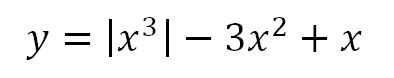
Gradient Descent needs a function and a starting point as input. Let’s define and plot a function:

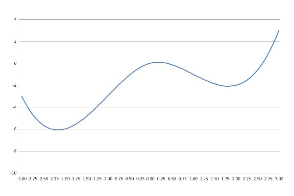
We can start at any desired point. Let’s start at x=1:

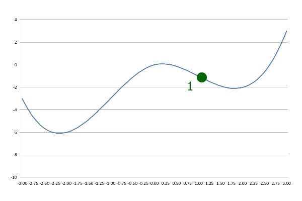
In the first step, Gradient Descent goes down the slope with a pre-defined step size:

Next, it goes further with the same step size. However, this time it ends up at a greater y than the last step:

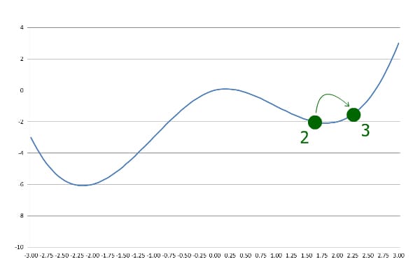
This indicates that the algorithm has passed the local minimum, so it goes backward with a lowered step size:

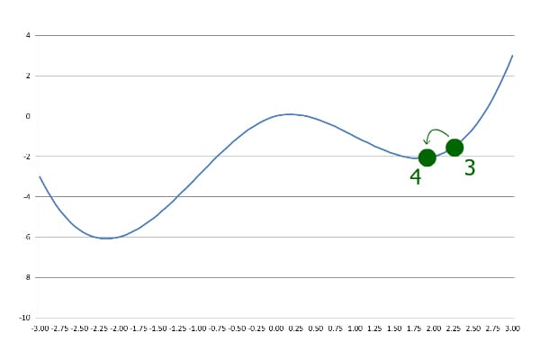
Subsequently, whenever the current y is greater than the previous y, the step size is lowered and negated. The iteration goes on until the desired precision is achieved.

As we can see, Gradient Descent found a local minimum here, but it is not the global minimum. If we start at x=-1 instead of x=1, the global minimum will be found.

5. Implementation in Java

There are several ways to implement Gradient Descent. Here we don’t calculate the derivative of the function to find the direction of the slope, so our implementation works for non-differentiable functions as well.

Let’s define precision and stepCoefficient and give them initial values:

double precision = 0.000001;
double stepCoefficient = 0.1;

In the first step, we don’t have a previous y for comparison. We can either increase or decrease the value of x to see if y lowers or raises. A positive stepCoefficient means we are increasing the value of x.

Now let’s perform the first step:

double previousX = initialX;
double previousY = f.apply(previousX);
currentX += stepCoefficient * previousY;

In the above code, f is a Function<Double, Double>, and initialX is a double, both being provided as input.

Another key point to consider is that Gradient Descent isn’t guaranteed to converge. To avoid getting stuck in the loop, let’s have a limit on the number of iterations:

int iter = 100;

Later, we’ll decrement iter by one at each iteration. Consequently, we’ll get out of the loop at a maximum of 100 iterations.

Now that we have a previousX, we can set up our loop:

while (previousStep > precision && iter > 0) {
    iter--;
    double currentY = f.apply(currentX);
    if (currentY > previousY) {
        stepCoefficient = -stepCoefficient/2;
    }
    previousX = currentX;
    currentX += stepCoefficient * previousY;
    previousY = currentY;
    previousStep = StrictMath.abs(currentX - previousX);
}

In each iteration, we calculate the new y and compare it with the previous y. If currentY is greater than previousY, we change our direction and decrease the step size.

The loop goes on until our step size is less than the desired precision. Finally, we can return currentX as the local minimum:

return currentX;

6. Conclusion

In this article, we walked through the Gradient Descent algorithm with a step-by-step illustration.

We also implemented Gradient Descent in Java. The code is available over on GitHub.

Persistence

REST