1. 简介
序列化是指将数据结构或对象转换为一串比特流,以便可以将其存储在文件或内存缓冲区中,或者通过网络传输。 未来我们可以通过反序列化这串比特流重建原始的数据结构或对象。
在本教程中,我们将介绍如何对一个二叉树进行序列化和反序列化。
2. 二叉树定义
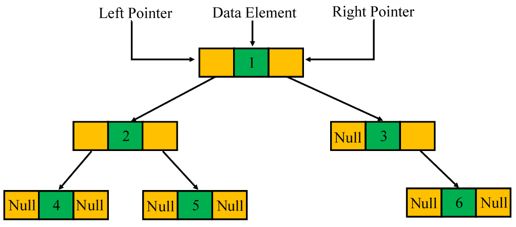
二叉树是一种每个节点最多有两个子节点的层级结构数据结构。 每个节点包含三部分:存储数据的元素,以及分别指向左子节点和右子节点的两个指针。如果某个子节点不存在,则用 null 表示:
二叉树有三种主要的遍历方式:前序、中序、后序。我们可以通过其中两种遍历结果组合来重建二叉树,比如前序 + 中序。
但本文将展示如何仅使用一种遍历方式完成序列化和反序列化。例如,我们可以使用前序遍历进行序列化,并使用相同方式反序列化。
3. 使用前序遍历序列化二叉树
我们可以使用前序遍历算法对二叉树进行序列化。 前序遍历的顺序是:先访问根节点,然后递归访问左子树和右子树。
例如,对上面的例子进行前序遍历的结果为:1, 2, 4, 5, 3, 6。
在序列化时,我们也要考虑 null 节点。我们可以用 # 来表示 null 节点。因此,前序序列变为:1, 2, 4, #, #, 5, #, #, 3, #, 6, #, #。
我们可以使用递归前序遍历实现序列化:
algorithm serializePreOrder(root, sequence):
    // INPUT
    //    root = the root node of the binary tree
    //    sequence = the sequence to append the serialization result
    // OUTPUT
    //    A serialization sequence of the binary tree

    if root is null:
        sequence <- sequence + "#"
    else:
        sequence <- sequence + root.data
        serializePreOrder(root.left, sequence)
        serializePreOrder(root.right, sequence)
该算法的时间复杂度和空间复杂度均为 **O(n)**,因为我们每个节点只访问一次,并且最多需要存储 2n 个 null 节点。
4. 使用前序遍历反序列化二叉树
我们也可以使用相同的前序算法将序列反序列化为二叉树。
algorithm deserializePreorder(sequenceIterator):
    // INPUT
    //    sequenceIterator = an iterator for the serialization sequence
    // OUTPUT
    //    The root node of the deserialized binary tree

    if not sequenceIterator.hasNext():
        return null
    data <- sequenceIterator.next()
    if data = "#":
        return null
    else:
        root <- create a new tree node with data
        root.left <- deserializePreorder(sequenceIterator)
        root.right <- deserializePreorder(sequenceIterator)
        return root

algorithm deserialize(sequence):
    // INPUT
    //    sequence = the serialization sequence of a binary tree
    // OUTPUT
    //    The root node of the deserialized binary tree

    sequenceIterator <- create an iterator for sequence
    return deserializePreorder(sequenceIterator)
这个过程和序列化类似,先构建根节点,再递归构建左右子树。遇到 # 就返回 null。
时间复杂度和空间复杂度均为 **O(n)**。
5. 使用后序遍历序列化二叉树
类似于前序遍历,我们也可以使用后序遍历对二叉树进行序列化。 后序遍历顺序是:先访问左子树,再访问右子树,最后访问根节点。
我们使用递归实现后序序列化:
algorithm serializePostOrder(root, sequence):
    // INPUT
    //    root = the root node of the binary tree
    //    sequence = the sequence to append the serialization result
    // OUTPUT
    //    A serialization sequence of the binary tree

    if root is null:
        sequence <- sequence + "#"
    else:
        serializePostOrder(root.left, sequence)
        serializePostOrder(root.right, sequence)
        sequence <- sequence + root.data
该算法的时间复杂度和空间复杂度也为 **O(n)**。
6. 使用后序遍历反序列化二叉树
与前序不同的是,后序的根节点位于序列的末尾。例如,上述例子的后序序列是:#, #, 4, #, #, 5, 2, #, #, #, 6, 3, 1。
为了反序列化后序序列,我们可以先反转整个序列,然后按照前序的方式进行反序列化,但要注意构建顺序是先右子树,再左子树:
algorithm deserializePostorder(sequenceIterator):
    // INPUT
    //    sequenceIterator = an iterator for the reversed serialization sequence
    // OUTPUT
    //    The root node of the deserialized binary tree

    if not sequenceIterator.hasNext():
        return null
    data <- sequenceIterator.next()
    if data = "#":
        return null
    else:
        root <- create a new tree node with data
        root.right <- deserializePostorder(sequenceIterator)
        root.left <- deserializePostorder(sequenceIterator)
        return root

algorithm deserialize(sequence):
    // INPUT
    //    sequence = the serialization sequence of a binary tree
    // OUTPUT
    //    The root node of the deserialized binary tree

    sequence <- reverse the sequence
    sequenceIterator <- create an iterator for the reversed sequence
    return deserializePostorder(sequenceIterator)
同样,时间复杂度和空间复杂度均为 **O(n)**。
7. 中序遍历的局限性
我们不能使用中序遍历对二叉树进行序列化和反序列化。
中序遍历的顺序是:先访问左子树,再访问根节点,最后访问右子树。这使得我们无法唯一确定根节点的位置。
例如,下面两棵树的中序遍历结果都为 #, 2, #, 1, #:
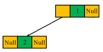
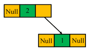
这说明中序遍历无法唯一还原二叉树结构,因此不适合用于序列化和反序列化。
8. 总结
✅ 在本教程中,我们介绍了两种可用于二叉树序列化和反序列化的算法:
- 前序遍历:直接使用前序序列化和反序列化
- 后序遍历:反转序列后,使用类似前序的方式反序列化
❌ 中序遍历则不适用,因为其序列无法唯一还原二叉树。
⚠️ 注意:所有算法的时间复杂度和空间复杂度均为 **O(n)**。