What Is the Difference Between Linear and Circular Convolution?

1. Introduction

In this tutorial, we’ll explore the concept of convolution, distinguishing between linear and circular convolution.

2. Linear Convolution: Intuitive Understanding and Mathematical Model

Convolution combines two functions to produce a third function, showing how one modifies the other.

In this section, we’ll offer an intuitive understanding of linear convolution before presenting its mathematical model.

2.1. Intuitive Understanding: A Bakery’s Delivery Schedule

Here, let’s use a bakery’s delivery schedule to understand the concept of linear convolution.

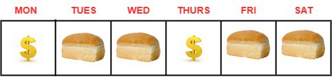
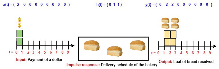
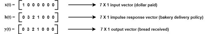
If we pay a dollar on monday, we get a loaf of bread on tuesday and wednesday in that order.  The next two figures illustrate this schedule and its timeline.

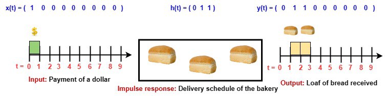
Here, is the amount we pay to the bakery (input), is the number of loaves we receive each day (output), and is the bakery’s delivery schedule (impulse response).

If we pay a dollar on the first and sixth days, we receive a loaf on the second, third, seventh, and eighth days based on the bakery’s schedule. The next figure illustrates this:

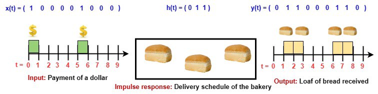
Regardless of when we pay, the bakery’s response remains consistent. This indicates that the bakery’s policy is unaffected by changes in time, making it a Time-Invariant system.

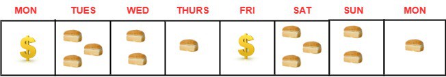
Let’s imagine another scenario. If the buyer pays one dollar to the baker two days in a row, what happens?

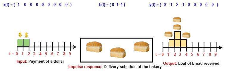
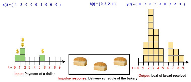
We discover that the loaves of bread stack upon one another and scale the output as we slide through the baker’s impulse response. The next figure also illustrates this stacking property:

Here, the buyer paid two dollars in one day. The output is stacked and scaled based on the bakery’s impulse response. This stacking and scaling property define a Linear system. Combining these properties, we conclude our bakery’s schedule is a Linear Time-Invariant (LTI) system.

Let’s consider another bakery with an LTI system and a different delivery policy: paying a dollar today gets you three loaves tomorrow, two loaves the next day, and one loaf on the third day:

Here is how this LTI system will look like on a timeline:

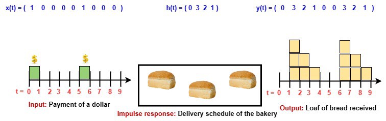
This is another LTI system timeline:

2.2. Forming and Interpreting the Vectors and Matrices

Let us capture all this information using vectors, matrices, and linear algebra.

We know that the matrix multiplication of and will yield .

Using our timeline analogy and the concepts of sliding, stacking, and scaling, we show how and behave as we shift the input over time.

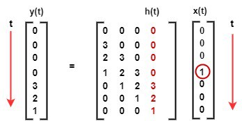
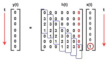
Starting with a simple input vector , here is how the matrix will look like:

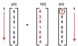
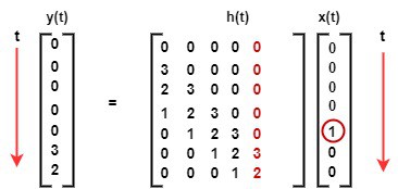
If we shift the input downward by one step, the impulse response also shifts downward by one step, resulting in the same output but shifting downward by one step. This is shown in the next figure:

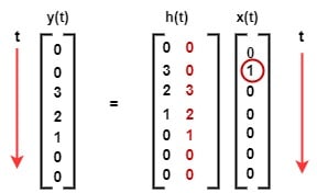
if we keep repeating this pattern for the other inputs, we obtain these patterns for and :

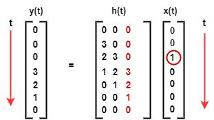
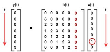
within each column of , we have its shifted version, as shown in the next figure:

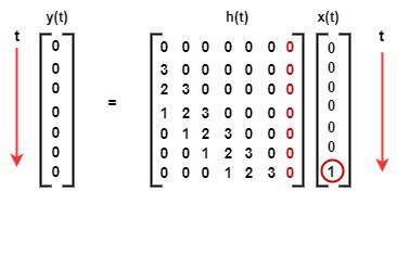
Along the row, we also get a copy of , but it’s a reflected and shifted version of as shown next:

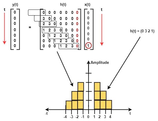
From our understanding of the pattern of the last two figures, we can generalize our matrix now as this:

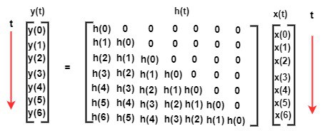
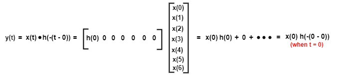
From matrix multiplication, we understand that the output vector is the dot product of the input vector and the row vector of the reflected and shifted impulse response. We express the output vector as a dot product of and :

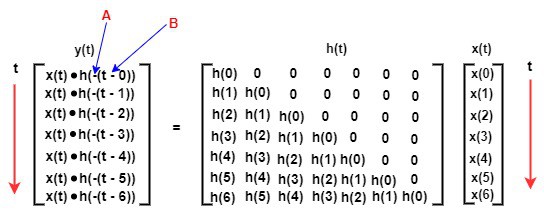
The negative sign at reflects the impulse response, while the negative sign at shifts it.

Let’s illustrate how translates to 

For the first row, , we have:

For the third row, we have:

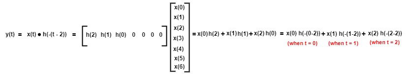
As time increases, so does the shift, indicating that the output is a function of the shift.

To avoid having in a generalized form, we replace the input time variable with and maintain the output time variable as .

With this, we obtain the generalized expression for the output vector:

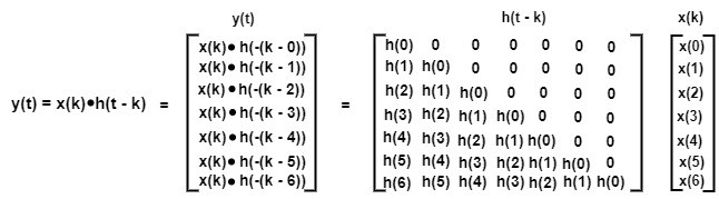
We can express the dot product explicitly with sigma notation:

To represent the system with a continuous function, we convert the sigma sum into an integral:

.

2.3. Mathematical Definition

Linear convolution combines two LTI sequences or time functions to produce a third sequence or function. It involves multiplying each sample of one function with the corresponding sample of the other function shifted by , then summing up the results over all possible values of .

In discrete LTI systems, the formula for convolution is:

   

In continuous-time LTI systems, it becomes:

   

The asterisk (*) denotes the convolution operator.

Now, let’s explore the various methods of computing linear convolution.

3. Linear Convolution: Methods of Computation

This article focuses on the short data sequences. Let’s take a look at an example:

3.1. An Example

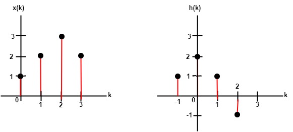
We are to determine the response of an LTI system whose input and impulse response are given as:

, and

.

To solve this, we note the following:

• Let the length of the first sequence be and the second sequence is . Then, the length of the output sequence is
• If the first sequence starts at and the second at , the output sequence will begin at and end at

For our example:

• , and , then, . will have a length of
• Also, , and , then, will start at , and ends at

Now, let’s investigate the graphical method.

3.2. The Graphical Method

Using the graphical method, we aim to visually overlap and shift sequences to compute their convolution by summing the products of their overlapping values.

We present the steps to follow in Table 1:

Steps

Process

1

Obtain the reverse sequence h(-k)

2

Shift h(-k) by n samples to get h(n-k). If n >= 0, h(-k) will be shifted to the right by n samples. But if n < 0, h(-k) will be shifted to the left by n samples

3

Perform the convolution sum, i.e., the sum of x(k) and h(n-k) to obtain y(n)

4

Repeat steps 1 to 3 for the next convolution value y(n)

In solving the problem using the graphical method, we first draw the graph of both sequences:

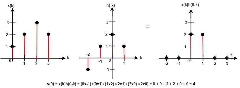
To obtain  at , we reverse to . Then, we multiply by and sum the products. The next plots show how we obtain :

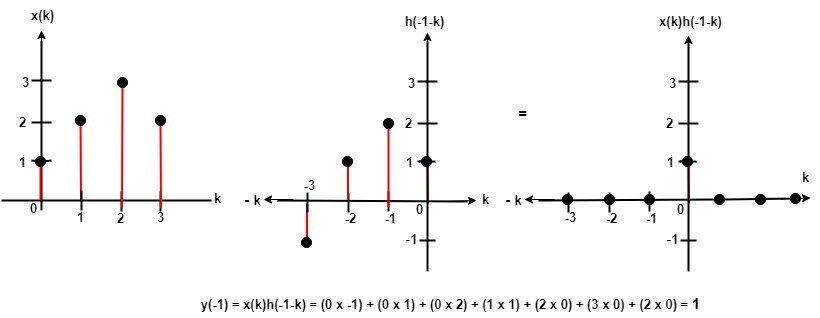
Our output starts at , so we need to obtain . To do this, we compute , shifting leftward. The next plots show this operation:

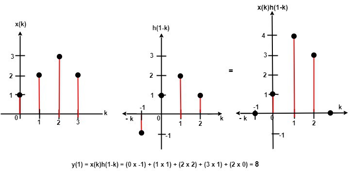
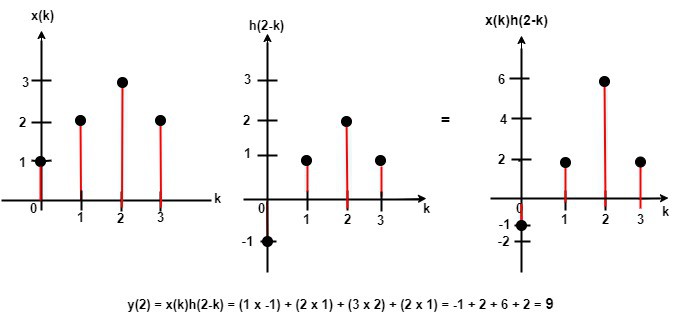
Next is to compute the output for by solving for shifting rightward. This operation is shown in the next plots:

For the output , its graph looks like this:

Here is the plot for :

for :

and here is for :

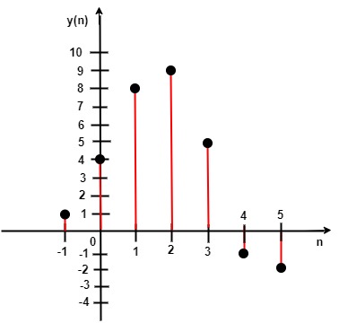
The output sequence and its graph is shown next:

,

Now, let’s attempt to solve this same given problem using the tabular method.

3.2. The Tabular Method

Using the tabular method, we systematically align and multiply sequences to compute their convolution step by step.

Table 2 provides the steps to follow:

Steps

Process

1

List the index k covering a sufficient range

2

List the input x(k)

3

Obtain the reversed sequence h(k), and align the rightmost element of h(n-k) to the leftmost element of x(k)

4

Cross-multiply and sum the non-zero overlap terms

5

Slide h(n-k) to the right by one step

6

Repeat step 4. Stop if all output values are zero or if required

Let’s now solve the given problem by following the steps, we show the result in Table 3:

k

-3

-2

-1

0

1

2

3

4

5

6

y(n)

x(k)

1

2

3

2

h(k)

1

2

1

-1

h(-k)

-1

1

2

1

h(-1-k)

-1

1

2

1

y(-1) = x(k)h(-1-k) = 0+0+0+1 = 1

h(0-k)

-1

1

2

1

y(0) = x(k)h(0-k) = 0+0+2+2 = 4

h(1-k)

-1

1

2

1

y(1) = x(k)h(1-k) = 0+1+4+3 = 8

h(2-k)

-1

1

2

1

y(2) = x(k)h(2-k) = -1+2+6+2 = 9

h(3-k)

-1

1

2

1

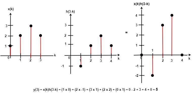
y(3) = x(k)h(3-k) = 0-2+3+4 = 5

h(4-k)

-1

1

2

1

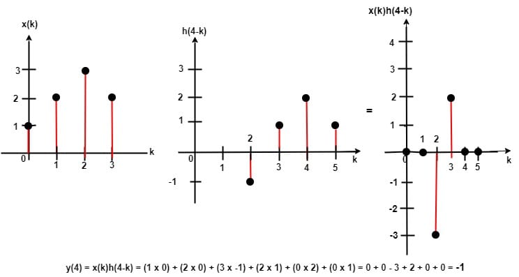
y(4) = x(k)h(4-k) = 0+0-3+2 = -1

h(5-k)

-1

1

2

1

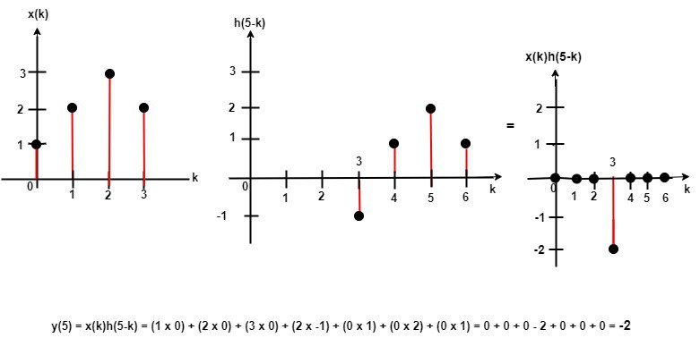
y(5) = x(k)h(5-k) = 0+0+0-2 = -2

Here is the output sequence:

,

This is the same as that of the graphical method.

Let’s look at the matrix method.

3.3. Matrix Method

We convert sequences into matrices using the matrix method to compute their convolution through matrix multiplication efficiently.

Table 4 provides the steps to follow:

Steps

Process

1

Arrange x(k) as a column

2

Arrange h(k) as a row

3

Obtain the element of a two-dimensional array by multiplying the corresponding row elements with the column elements

4

The sum of the diagonal element gives the samples y(n)

Let’s solve the given problem using these steps:

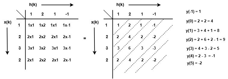
Here is the output sequence:

,

The same as that of the graphical and tabular methods.

4. Circular Convolution

Using circular convolution, we compute the convolution of two sequences assuming they are periodic, resulting in an output of the same length.

The mathematical formula for circular convolution is:

   

for   

Let’s explore the short sequence methods.

4.1. Concentric Circle Method

Using the concentric circle method, we visually align and rotate sequences to compute their circular convolution efficiently.

Table 5 provides the steps to follow:

Steps

Process

1

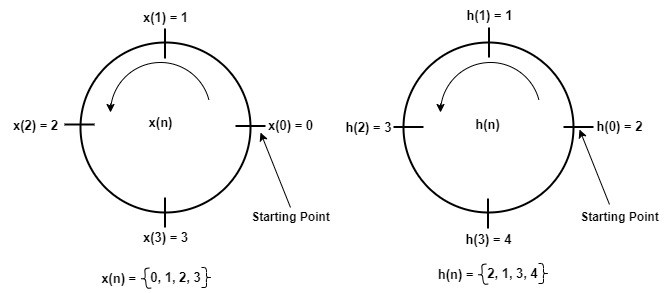
Draw two concentric circles, one will represent x(n), and the other h(n)

2

Place the elements x(n) on the inner circle and h(n) on the outer circle at corresponding positions

3

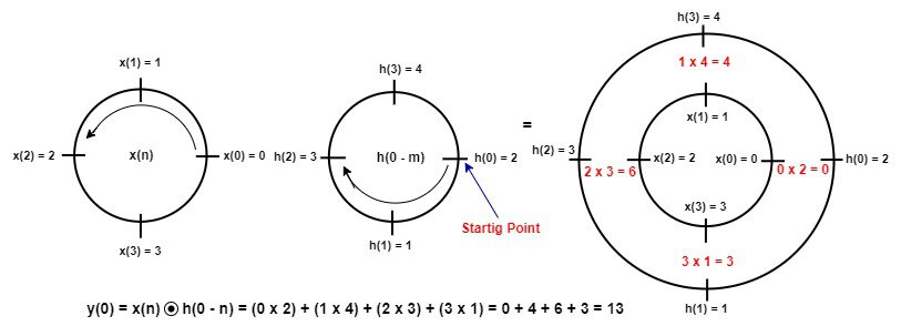
Align the first element of x(n) with the first element of h(n)

4

For the current alignment, multiply corresponding elements of x(n) and h(n), then sum these products to het y(n)

5

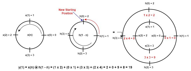
Rotate the outer circle h(n) one position clockwise

6

Repeat the multiplication and summation process for each new alignment to get other output y(n)

7

Continue rotating the outer circle and computing sums until you have completed N rotations, generating all elements of y(n)

8

The sequence y(n) represents the circular convolution result

We illustrate this method with an example:

4.2. An Example

We are to determine the response of an LTI system whose input and impulse response are given as:

, and,

.

Here’s the solution.

Given sequences and with length , the equation is:

First, we draw two circles, one for and the other for , plotting their elements in an anti-clockwise direction:

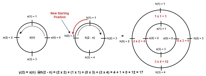
To calculate , we substitute into our circular convolution equation:

The sequence is the circular folding of , obtained by plotting clockwise. To obtain , we plot and on two concentric circles, with on the inner circle and on the outer circle and then multiply and sum each point. The next figure shows this process:

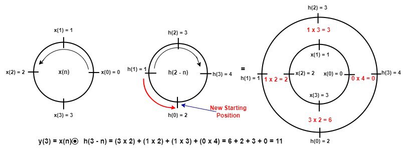
To obtain , we shift anti-clockwise by one sample. We then plot the new sequence clockwise and apply multiplication and summation, as shown in the next figure:

Here is the output :

And here is for output :

Here is the resultant output sequence :

.

Now, let’s look at the matrix method.

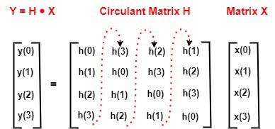
4.3. Matrix Method

We convert sequences into circulant matrices using the matrix method to compute their circular convolution through matrix multiplication efficiently.

Table 6 provides the steps to follow:

Steps

Process

1

Define the sequence x(n) and h(n), each of length N

2

Construct a circulant matrix H using the sequence h(n)

3

Populate the circulant matrix H such that each row is a cyclic permutation of h(n)

4

Arrange the sequence x(n) as a column vector X

5

Perform the matrix multiplication Y = H . X

6

The resulting vector Y represents the circular convolution y(n)

7

The sequence y(n) is the output of the circular convolution

We illustrate this method with the same example as before.

, and,

.

The matrix will have this format:

Let’s fill in the sequences into the matrix, we have:

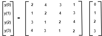
Now, let’s perform matrix multiplication and summation:

Here is the output sequence:

,

It’s the same as the concentric circle method.

5. Interplay Between Linear and Circular Convolution.

In this section, we demonstrate how linear convolution extends sequences and how circular convolution handles periodic sequences efficiently, showcasing their interplay and equivalence under specific conditions.

Let’s perform the following operations on the sequences and to illustrate the interplay between linear and circular convolution:

• Linear convolution
• Circular convolution
• Converting linear convolution into circular convolution
• Linear convolution using circular convolution

To perform linear convolution with and , the lengths are and , giving . Using the matrix method, the output is .

For circular convolution, both sequences must be the same length . Since has length and has length , we append a zero to , making . Using the matrix method, the output is .

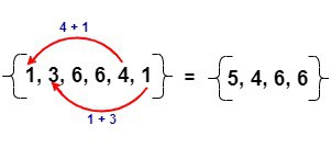
To convert linear convolution to circular convolution, subtract from : . The value means that we will add the last two elements of the linear convolution sequence to the first two elements as illustrated in the next figure:

To perform linear convolution using circular convolution, we append zeros to both sequences to make them equal in length. First, we determine the output sequence’s length, . This means that we append   zeros to and zeros to to make each sequence a length of .

Thus, and .

Using the circular matrix method, the output is , matching the linear convolution result.

6. Differences Between Linear and Circular Convolution

Based on all our discussion in this article, here are the differences between linear and circular convolution:

Linear Convolution

Circular Convolution

It considers the full length of the resulting sequence

It warps around the sequence, assuming periodicity

Its output length is N + M -1 if x(n) and h(n) is of length N and M respectively

Its output has the same length as x(n) and h(n)

The result is not periodic

The result is periodic with period N

It requires zero padding to avoid edge effects

It doesn’t need zero padding as it is periodic

Convolution in the time domain corresponds to multiplication in the frequency domain with zero padding to the length of N + M – 1

Convolution in the time domain corresponds to multiplication in the frequency domain without zero padding

Direct computation is O(NM), but can use FFT for O((N + M)log(N + M))

Efficiently computed using FFT with complexity O(NlogN)

Requires zero padding before applying the DFT to avoid aliasing

Directly corresponds to the multiplication of DFTs of sequences

Exists if the sequences are invertible, but may not be straightforward

Circular deconvolution can be applied if the sequences are invertible in the circular sense

Typically used in applications where the length of the resulting sequence matters, like in analogue signal processing and filtering

Often used in digital signal processing, especially in FFT-based methods, where computational efficiency is crucial

7. Conclusion

In this article, we analyzed the intuition behind linear and circular convolution, their mathematical models, and various types. By focusing on short sequences, we provided examples to clarify these concepts. Finally, we listed the key differences between linear and circular convolution.