神经网络权重衰减和学习率的区别

1. Introduction

Neural networks have become a cornerstone of modern machine learning and artificial intelligence, powering applications ranging from image recognition and natural language processing to autonomous driving and financial forecasting.

Two of the most critical hyperparameters in neural network training are weight decay and learning rate. These parameters play crucial roles in the optimization process, helping to prevent overfitting and ensuring that the model converges to a solution.

In this article, we’ll discuss the main differences between weight decay and learning rate.

2. Understanding Weight Decay

Weight decay, also known as regularization, is a crucial technique used in the training of neural networks to prevent overfitting and enhance the generalization of the model. Overfitting occurs when a model learns the noise and details in the training data to the extent that it negatively impacts the model’s performance on new data. Weight decay addresses this issue by adding a regularization term to the loss function, which penalizes large weights.

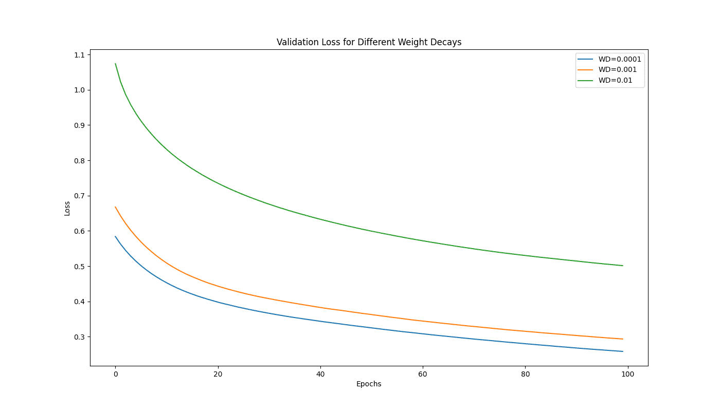
This plot shows the effect of varying weight decay values (0.0001, 0.001, and 0.01) on the validation loss, highlighting how increased regularization through higher weight decay values can help in reducing overfitting:

Weigh decay example

2.1. Mathematical Approach

Weight decay refers to a regularization technique where a penalty proportional to the square of the magnitude of the weights is added to the loss function.

Mathematically, if $L_0(\theta)$ represents the original loss function (e.g., mean squared error for regression or cross-entropy loss for classification), the loss function with weight decay becomes:

(1) $\begin{equation*} L(\theta)= L_0(\theta) + \frac{\lambda}{2} \|\theta\|^2 \end{equation*}$

Here, $\theta$ denotes the vector of weights, and $\lambda$ is a hyperparameter controlling the strength of the penalty. The term $||\theta||^2$ is the L_2 norm of the weight vector, calculated as the sum of the squares of all individual weights.

2.2. Benefits of Using Weight Decay

The primary purpose of weight decay is to prevent the model from becoming overly complex and capturing noise from the training data. By penalizing large weights, weight decay encourages the network to maintain smaller weights, leading to simpler models that are less likely to overfit. This results in better generalization performance, where the model performs well on the training data and unseen data.

So, the weight decay acts as a regularizer by discouraging the model from relying too heavily on any single feature or input data point. Moreover, it helps stabilize the training process by preventing the weights from growing too large. Furthermore, it improves the model’s ability to generalize to new, unseen data, leading to better performance in real-world applications.

2.3. When to Use Weight Decay

Weight decay is particularly useful in scenarios where the training dataset is relatively small compared to the number of model parameters, increasing the risk of overfitting. When the model exhibits high variance, where performance significantly varies between training and validation datasets.

Moreover, it can be useful when the data contains noise or irrelevant features that the model might otherwise learn during training.

3. Understanding Learning Rate

The learning rate is a critical hyperparameter in neural network training that determines the step size during the optimization process. It controls how much to adjust the model’s weights with respect to the loss gradient at each iteration of the training. Proper tuning of the learning rate is essential for efficient training and good performance.

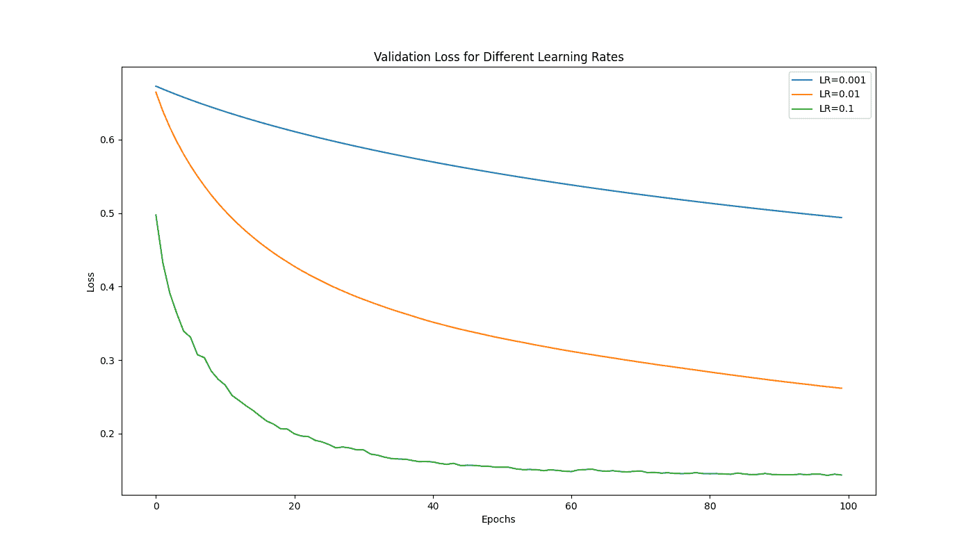
The plot demonstrates the impact of different learning rates (0.001, 0.01, and 0.1) on the validation loss during the training of a neural network, illustrating how a higher learning rate can lead to faster convergence but may also cause more fluctuation:

Learning Rate Example

3.1. Mathematical Approach

The learning rate is often denoted as $\eta$ or $\alpha$ , is a scalar value that scales the magnitude of weight updates in the gradient descent optimization algorithm. During training, the weights of the neural network are updated in the direction of the negative gradient of the loss function to minimize the loss. The weight update rule can be expressed mathematically as:

(2) $\begin{equation*} \theta_{t+1} = \theta_t - \eta \nabla L(\theta_t) \end{equation*}$

Here, $\theta_t$ represents the weights at iteration , $\eta$ is the learning rate, and $\nabla L(\theta_t)$ is the gradient of the loss function with respect to the weights.

3.2. Benefits of Using Weight Decay

The learning rate plays a pivotal role in determining the speed and stability of the training process. Its value impacts the following aspects:

It offers convergence speed as a larger learning rate can accelerate the training process by taking larger steps towards the minimum of the loss function. However, if the learning rate is too large, the optimization process may overshoot the minimum, leading to divergence or oscillations.

A lower learning rate ensures stable convergence by taking smaller steps, but it can make the training process slow and prone to getting stuck in local minima and, therefore, offer stability. An appropriately chosen learning rate balances the trade-off between fast convergence and stable, efficient optimization, leading to better performance.

3.3. Examples of Common Learning Rates

Choosing a constant learning rate throughout the training process may not always be optimal. Various learning rate schedules can be employed to improve training efficiency:

Constant Learning Rate: A fixed learning rate throughout the training process
Step Decay: The learning rate is reduced by a factor at fixed intervals. For example, reducing the learning rate by half every 10 epochs
Exponential Decay: The learning rate decreases exponentially over epochs. The formula is $\eta_t = \eta_0 \cdot \exp(-kt)$ , where $\eta_0$ is the initial learning rate, is the decay rate, and is the epoch number
Adaptive Learning Rates: Algorithms like AdaGrad, RMSprop, and Adam adjust the learning rate for each parameter individually based on the historical gradients. These methods can adaptively decrease the learning rate as training progresses

4. Case Studies and Examples

When choosing the right weight decay and learning rate, practical considerations and empirical experimentation are key. The optimal settings depend on various factors, including the model’s complexity, the dataset’s size, and the specific task at hand. Generally, weight decay values range from $10^{-4}$ to $10^{-2}$ while learning rates are between $10^{-3}$ and $10^{-1}$ .

During training, we might observe that the model initially converges well but then overfits. In this case, increasing the weight decay can help by penalizing large weights more strongly. Conversely, if the model’s convergence is too slow, increasing the learning rate or employing learning rate schedules like step decay or exponential decay can be beneficial.

For instance, a step decay that reduces the learning rate by a factor of 0.1 every 20 epochs can help refine the model’s performance as it approaches a minimum.

Visualizing training and validation loss curves can provide insights into the effectiveness of these hyperparameters.

5. Interaction Between Weight Decay and Learning Rate

Weight decay and learning rate work together to shape the trajectory of the optimization process. The learning rate determines the size of the steps taken during gradient descent, while weight decay acts as a regularizing force that penalizes large weights, promoting smaller, more generalizable models.

When the learning rate is high, the weight updates are large, and the influence of weight decay is magnified. In this scenario, if the weight decay is too strong, it can overly penalize the weights, leading to underfitting where the model fails to capture the underlying patterns in the data.

Conversely, suppose the learning rate is too low. In that case, the regularizing effect of weight decay might be insufficient to prevent overfitting, as the model might converge too slowly or get stuck in local minima.

6. Conclusion

In this article, we gained a deep understanding of weight decay and learning rate, coupled with careful tuning and validation, which is essential for training effective neural network models. By leveraging these insights, we can build models that not only achieve high performance on training data but also exhibit strong generalization to new, unseen data.

Persistence

REST

Security