1. 简介
本文将介绍如何在三种图遍历算法中追踪路径:深度优先搜索(DFS)、广度优先搜索(BFS)和迪杰斯特拉算法(Dijkstra’s Algorithm)。重点在于展示这些算法在找到目标节点的同时,如何返回完整的路径,而不仅仅是路径长度。
虽然 DFS 本身不能保证找到最短路径,但在某些实现中仍可追踪路径;BFS 则在无权重图中能保证找到最短路径;而 Dijkstra 算法则适用于带正权重图的最短路径查找。
2. 递归深度优先搜索中的路径追踪
DFS 有两种实现方式:递归和迭代。在递归版本中追踪路径相对简单,只需在找到目标节点后,将路径逐层返回即可。
以下是一个递归 DFS 的伪代码示例:
algorithm DepthFirstSearch(s, target):
    // INPUT
    //    s = 起始节点
    //    target = 判断是否为目标节点的函数
    // OUTPUT
    //    从 s 到目标节点的路径

    if target(s):
        return [s]

    for v in neighbors(s):
        path <- DepthFirstSearch(v, target)

        if path != empty set:
            path <- prepend v to path
            return path

    return empty set
2.1 示例
考虑如下图结构:
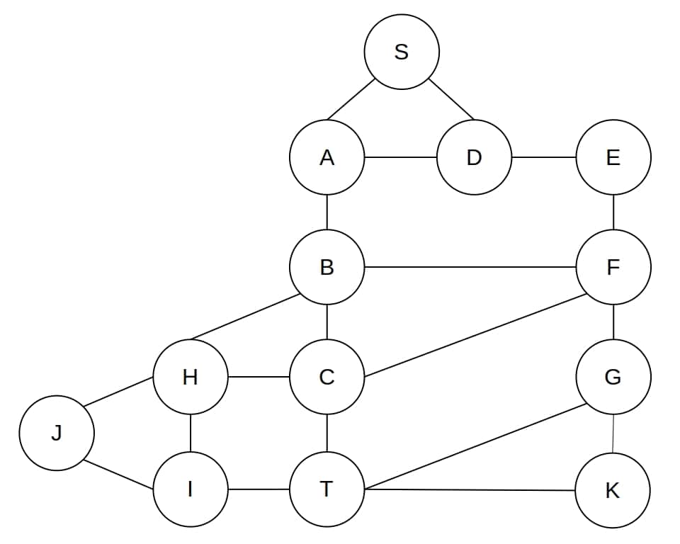
我们希望从节点 S 到 T 找到一条路径。DFS 会按顺序展开子节点,最终找到路径 [S, A, B, C, T]:
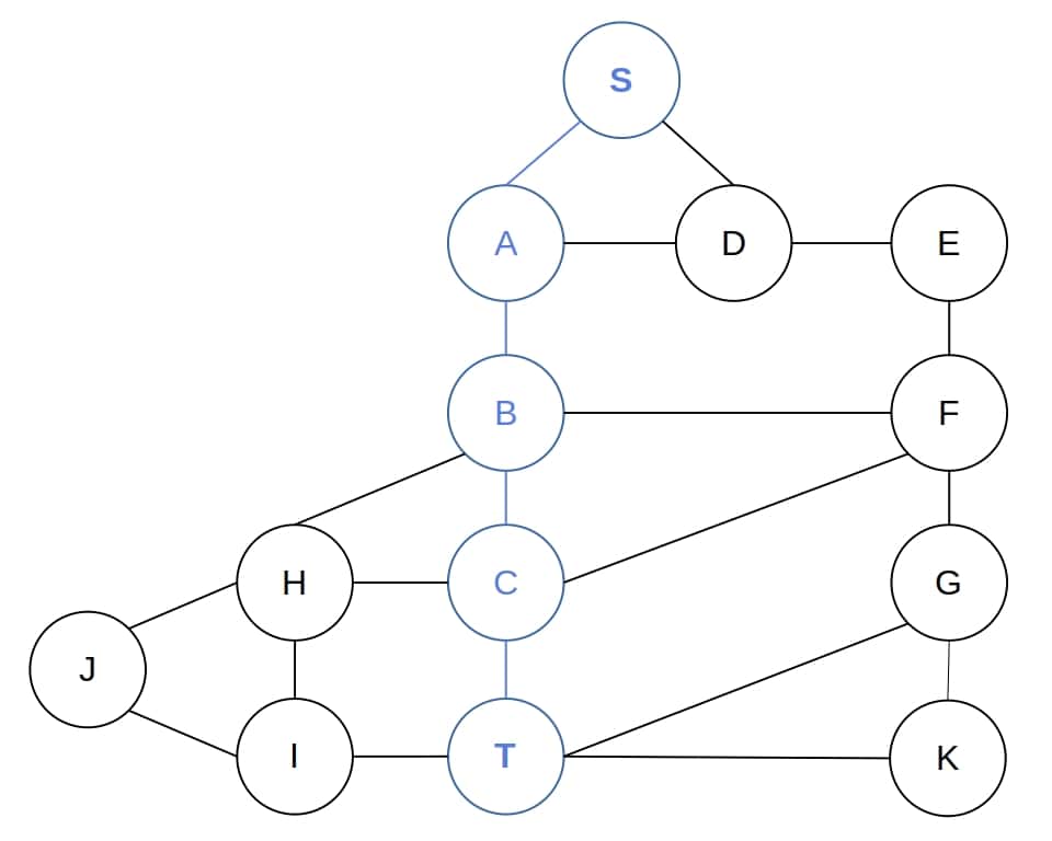
虽然在这个例子中找到了最短路径,但需要注意的是,DFS 并不总是能找到最短路径,路径的准确性取决于子节点的访问顺序。
3. 迭代深度优先搜索中的路径追踪
递归 DFS 在某些场景下可能效率不高,因此我们常使用迭代实现。但迭代方式中路径追踪稍复杂,通常有两种方式:
- 记录父节点:通过记录每个节点的父节点,在找到目标节点后回溯路径。
- 保存完整路径:在搜索过程中直接保存每条路径,一旦找到目标节点即可直接返回。
3.1 记录父节点关系
algorithm IterativeDepthFirstSearchWithPathTracing(s, target, neighbors):
    // INPUT
    //    s = 起始节点
    //    target = 目标判断函数
    // OUTPUT
    //    从 s 到目标节点的路径

    if target(s):
        return s

    frontier <- 一个 LIFO 队列,初始只包含 s
    explored <- 一个空集合
    memory <- 用于记录父节点关系的结构
    Set s.parent <- null

    while frontier is not empty:
        u <- pop 最近加入的节点
        add u to explored

        for v in neighbors(u):
            v.parent <- u
            if u not in explored or frontier:
                if target(v):
                    path <- reconstruct path from s to v using memory
                    return path
                add v to frontier

    return empty set
3.2 路径重建
通过父节点回溯路径:
algorithm BackwardPathReconstruction(s, t, memory):
    // INPUT
    //    s = 起始节点
    //    t = 目标节点
    //    memory = 父节点记录结构
    // OUTPUT
    //    从 t 到 s 的路径

    path <- []
    u <- t

    while u != null:
        path.prepend(u)
        u <- memory[u]

    return path
若需要从 s 到 t 的顺序,可将路径反转:
algorithm ForwardPathReconstruction(s, t, memory):
    // INPUT
    //    s = 起始节点
    //    t = 目标节点
    //    memory = 父节点记录结构
    // OUTPUT
    //    从 s 到 t 的路径

    stack <- []
    u <- t

    while u != null:
        push u to stack
        u <- memory[u]

    path <- []
    while stack not empty:
        u <- pop from stack
        path.append(u)

    return path
3.3 父节点记录结构的实现
可以使用指针或哈希表来记录父节点关系:
- 每个节点保存一个
parent指针 - 使用数组或哈希表,以节点 ID 为键,存储其父节点 ID
例如:
int[] parent = new int[totalNodes];
parent[0] = -1; // root node
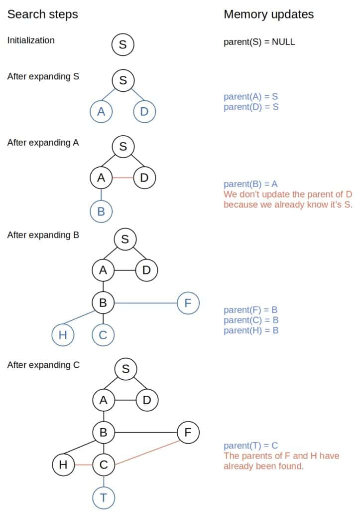
3.4 示例
以下是一个迭代 DFS 的路径追踪过程示意图:
3.5 直接保存路径
另一种方式是在迭代过程中直接保存路径:
algorithm IterativeDFSWithPathMemorization(s, target, neighbors):
    // INPUT
    //    s = 起始节点
    //    target = 目标判断函数
    // OUTPUT
    //    从 s 到目标节点的路径

    if target(s):
        return [s]

    frontier <- 一个 LIFO 队列,初始包含 (s, [s])
    explored <- 一个空集合

    while frontier not empty:
        (u, path) <- pop from frontier
        add u to explored

        for v in neighbors(u):
            new_path <- path + [v]
            if v not in explored or frontier:
                if target(v):
                    return new_path
                add (v, new_path) to frontier

    return empty set
这种方式虽然直观,但内存开销较大,因为每个节点都保存了完整的路径。
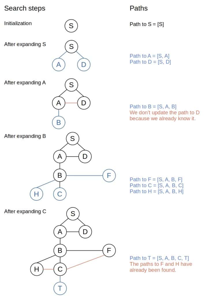
3.6 示例
路径追踪过程示意如下:
4. 广度优先搜索中的路径追踪
BFS 和 DFS 的路径追踪方式类似,但 BFS 使用 FIFO 队列,因此更适合寻找最短路径。
4.1 示例
BFS 从 S 到 T 的路径查找过程如下:
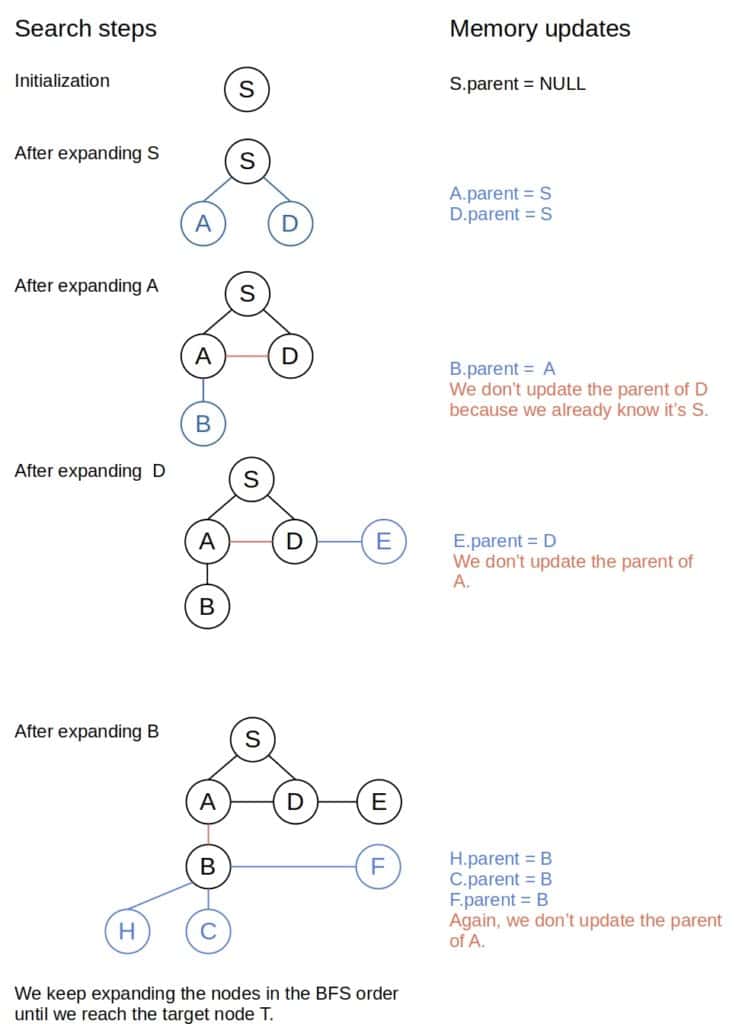
路径重建与 DFS 相同,使用父节点回溯即可:
algorithm BreadthFirstSearch(s, target, neighbors):
    // INPUT
    //    s = 起始节点
    //    target = 目标判断函数
    // OUTPUT
    //    从 s 到目标节点的路径

    if target(s):
        return [s]

    frontier <- FIFO queue with s
    explored <- empty set
    s.parent <- null
    t <- null

    while frontier not empty:
        u <- pop oldest node
        add u to explored

        for v in neighbors(u):
            v.parent <- u
            if v not in explored or frontier:
                if target(v):
                    t <- v
                    break
                add v to frontier
        if target(v):
            break

    if t is null:
        return empty set
    else:
        return reconstruct path from s to t
5. 迪杰斯特拉算法中的路径追踪
Dijkstra 算法用于带权图中的最短路径查找,其路径追踪方式与 BFS 类似,但需要维护一个 prev 数组来记录每个节点的前驱节点。
algorithm Dijkstra(s, G):
    // INPUT
    //    s = 起始节点
    //    G = 图结构
    // OUTPUT
    //    dist = 每个节点的最短距离
    //    prev = 前驱节点数组

    queue <- 一个最小优先队列
    dist <- 初始化为无穷大
    prev <- 初始化为 null

    dist[s] <- 0
    for each node v in G:
        add v to queue with priority dist[v]

    while queue not empty:
        u <- extract min from queue
        for v in neighbors(u):
            if dist[u] + weight(u, v) < dist[v]:
                dist[v] <- dist[u] + weight(u, v)
                prev[v] <- u
                update v's priority in queue

    return (dist, prev)
路径重建方式如下:
algorithm BackwardPathReconstruction(s, t, prev):
    // INPUT
    //    s = 起始节点
    //    t = 目标节点
    //    prev = 前驱数组
    // OUTPUT
    //    从 t 到 s 的路径

    path <- []
    u <- t

    while u != null:
        path.prepend(u)
        u <- prev[u]

    return path
6. 总结
| 算法 | 路径追踪方式 | 是否保证最短路径 |
|---|---|---|
| DFS(递归) | 递归返回路径 | 否 |
| DFS(迭代) | 父节点记录或路径保存 | 否 |
| BFS | 父节点记录 | 是(无权图) |
| Dijkstra | 前驱数组记录 | 是(带权图) |
✅ 建议:
- 若图无权重,且需最短路径,优先使用 BFS
- 若图有权重,使用 Dijkstra 并记录前驱节点
- DFS 适用于路径存在性判断或非最短路径问题
⚠️ 注意:DFS 和迭代 DFS 的路径准确性依赖于节点访问顺序,实际应用中应根据需求选择合适的方式。