在一致代价搜索算法中获取路径

1. 概述

在本文中，我们将讨论在一致代价搜索（Uniform Cost Search, UCS） 算法中如何获取从起点到终点的最短路径。

UCS 是一种用于寻找加权图中两个节点之间最小代价路径的算法，它本质上是 Dijkstra 算法的一个变体。虽然 UCS 可以轻松计算出最小代价，但默认情况下它不保留路径信息。因此，本文将重点介绍两种在 UCS 中获取完整路径的方法：

朴素方法（Naive Approach）：直接保存每个节点的完整路径
优化方法（Optimized Approach）：仅记录每个节点的父节点，最后通过回溯构造路径

我们还将通过一个简单图示说明问题，并对比两种方法的时间和空间复杂度。

2. 问题定义

我们给定一个图 G，包含 V 个节点和 E 条边，每条边都有一个权重表示代价。此外，我们还知道两个节点：

S：起点（Source）
D：终点（Destination）

我们的任务是使用 UCS 算法找出从 S 到 D 的最小代价路径。

示例图示

假设我们有如下图结构，S = 1，D = 4：

WeightedGraph

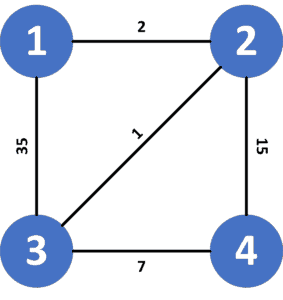
可能的路径有：

1 → 2 → 4，代价 = 17
1 → 2 → 3 → 4，代价 = 10 ✅
1 → 3 → 4，代价 = 42
1 → 3 → 2 → 4，代价 = 51

UCS 会找到代价最小的路径：1 → 2 → 3 → 4，代价为 10。

3. 朴素方法

3.1 核心思想

在每次更新节点代价时，同时更新其对应的完整路径。也就是说，我们维护两个数组：

cost[]：记录从起点到当前节点的最小代价
path[]：记录从起点到当前节点的路径（节点列表）

当发现更小代价的路径时，就将当前节点的路径设置为父节点的路径加上自己。

3.2 实现代码

List<Integer> naiveApproach(int V, List<List<Edge>> G, int S, int D) {
    int[] cost = new int[V];
    Arrays.fill(cost, Integer.MAX_VALUE);
    List<List<Integer>> path = new ArrayList<>(V);
    for (int i = 0; i < V; i++) path.add(new ArrayList<>());
    
    PriorityQueue<Integer> pq = new PriorityQueue<>(Comparator.comparingInt(i -> cost[i]));
    cost[S] = 0;
    path.get(S).add(S);
    pq.add(S);

    while (!pq.isEmpty()) {
        int current = pq.poll();
        for (Edge edge : G.get(current)) {
            int child = edge.to;
            int newCost = cost[current] + edge.weight;
            if (newCost < cost[child]) {
                cost[child] = newCost;
                path.get(child).clear();
                path.get(child).addAll(path.get(current));
                path.get(child).add(child);
                pq.add(child);
            }
        }
    }
    return path.get(D);
}

⚠️ 注意：path[child].addAll(path[current]) 必须是深拷贝，不能只是引用。

3.3 复杂度分析

时间复杂度：O(E + V log V + E * V)
因为每次更新都需要复制路径，路径长度可达 V，总共可能更新 E 次
空间复杂度：O(V^2)
每个节点的路径长度最多是 V，总共有 V 个节点

✅ 优点：实现直观
❌ 缺点：性能差，内存消耗高

4. 优化方法

4.1 核心思想

不直接保存路径，而是只记录每个节点的父节点（parent）。最后通过不断回溯父节点构造完整路径。

这种方式避免了频繁复制路径列表，大幅提升了性能和内存效率。

4.2 实现代码

List<Integer> optimizedApproach(int V, List<List<Edge>> G, int S, int D) {
    int[] cost = new int[V];
    Arrays.fill(cost, Integer.MAX_VALUE);
    int[] parent = new int[V];
    Arrays.fill(parent, -1); // -1 表示没有父节点
    
    PriorityQueue<Integer> pq = new PriorityQueue<>(Comparator.comparingInt(i -> cost[i]));
    cost[S] = 0;
    pq.add(S);

    while (!pq.isEmpty()) {
        int current = pq.poll();
        for (Edge edge : G.get(current)) {
            int child = edge.to;
            int newCost = cost[current] + edge.weight;
            if (newCost < cost[child]) {
                cost[child] = newCost;
                parent[child] = current;
                pq.add(child);
            }
        }
    }

    // 构造路径
    List<Integer> path = new ArrayList<>();
    int node = D;
    while (node != -1) {
        path.add(0, node); // 插入到列表开头
        node = parent[node];
    }
    return path;
}

4.3 复杂度分析

时间复杂度：O(E + V log V)
与标准 UCS 一致
空间复杂度：O(V)
只需额外一个 parent[] 数组

✅ 优点：性能好，内存低
✅ 推荐使用方式

5. 总结

方法	时间复杂度	空间复杂度	是否推荐
朴素方法	`O(E + V log V + EV)`	`O(V^2)`	❌
优化方法	`O(E + V log V)`	`O(V)`	✅

⚠️ 踩坑提醒：在实际项目中，尤其是图较大时，千万不要使用朴素方法，否则可能因为频繁拷贝路径导致性能急剧下降甚至内存溢出。

✅ 推荐做法：使用父节点回溯方式来构造路径，这是标准 UCS 实现中最常用、最高效的做法。

Persistence

REST

Security