How Does the Null Hypothesis Work?

1. Introduction

In this tutorial, we’ll explain the role of null hypotheses in standard statistical tests.

2. Statistical Tests

Let’s say we want to check how a new, recently proposed teaching method using generative AI affects students’ quiz results. To do this, we teach one class using the new AI-powered method and another using the good old presentation slides. To ensure a fair comparison, we choose the classes with equally talented students and instruct them to use the same textbook.

After scoring the quiz, we can be tempted to compute the mean scores in both classes to see which one is better. However, if we want to generalize the conclusions, we need to use statistics. The two classes we scored in this experiment are just two samples of the entire student population. So, the results might differ if the same experiment was conducted with different students. Statistical tests help us quantify this uncertainty and draw general conclusions with high confidence (if we conduct them correctly).

Usually, statistical tests have two hypotheses: the null and the alternative.

The null hypothesis is the hypothesis of “no effect,” i.e., the hypothesis opposite to the effect we want to test for. In contrast, the alternative hypothesis is the one positing the existence of the effect of interest.

3. Effects and Null Hypothesis

The effect depends on our research question. In our example, we want to check the efficacy of a new method, so we’re interested in the score difference. We must formulate the effect using quantifiable and measurable parameters to test it statistically.

Formally, let $\theta$ be the parameter we want to test. That can be the mean difference between the scores we get using the two methods. However, we’re referring to the population means, not sample averages. For instance, the mean score we get in the class taught using the old method is a sample mean $\widehat{S}_{old}$ , and the same goes for $\widehat{S}_{new}$ . In contrast, the means we’d get if we could teach all the students using these methods are the population means $\mu_{old}$ and $\mu_{new}$ .

So, if one method is better than the other, $\theta$ will be different from zero, and that’s our alternative hypothesis:

$[H_a: \theta = \mu_{old} - \mu_new} \neq 0]$

The opposite of H_a is that the mean scores are the same, i.e., that there is no effect, which is our null hypothesis H_0 :

$[H_0: \theta = \mu_{old} - \mu_{new} = 0]$

3.1. The Special Role of the Null Hypothesis

Rejecting H_0 in favor of H_a is justifiable if our test is calibrated to reject a true null rarely.

Formally, let be the statistic of the test to check if $H_0: \theta = \theta_0$ holds and let higher values be less compatible with H_0 . The value of $\theta_0$ corresponds to “no effect.” In our example with score difference, $\theta_0$ is 0.

Let t^* be the value of computed using our samples. The p-value of t^* is:

$[P(T \geq t^* \mid \theta = \theta_0)]$

Rejecting $\boldsymbol{H_0}$ if the $\boldsymbol{p}$ -value is lower than $\boldsymbol{\alpha}$ (usually 1% or 5%) means that our long-term frequency of rejecting true nulls will not exceed $\boldsymbol{\alpha}$ . The caveat is that every statistical test has implicit or explicit assumptions about the tested parameter(s). If the real world substantially deviates from the assumptions, we’ll be unable to limit the error rate from above.

The definition of the -value reveals that we use the null hypothesis to derive the distribution of the test statistic. Most of the time, it’s easier to analytically derive the distribution if we assume that there is no effect (which usually corresponds to the tested parameter $\theta$ being equal to 0).

3.2. The Nature of Scientific Proofs

The asymmetry between the null and alternative is evident in how we act depending on the test results. We’re usually interested in proving an effect. However, we behave as if that’s true only if the results are highly incompatible with the null hypothesis, as it isn’t sufficient that they are compatible with the alternative.

This means that the null acts as our default reality model, which is the one already in place or of lower risk. For instance, if we have a well-tested and very efficient teaching method, we don’t have much incentive to change it unless the new one is substantially better. Similarly, there’s more risk in erroneously recommending the use of an inefficient or harmful drug than not detecting the efficacy of an efficient one, so having a no-effect hypothesis as a default makes sense.

Therefore, we don’t need convincing to behave as if the null is true. It’s the job of the alternative hypothesis to convince us to act otherwise.

3.3. Effect Formulation

There’s more than one way to formulate the effect of interest. The choice of formulation implicitly defines assumptions about the populations. For instance, we defined the effect as a non-zero difference of means. However, the score distributions need to have the same shape for the difference in means to indicate the distributions are different:

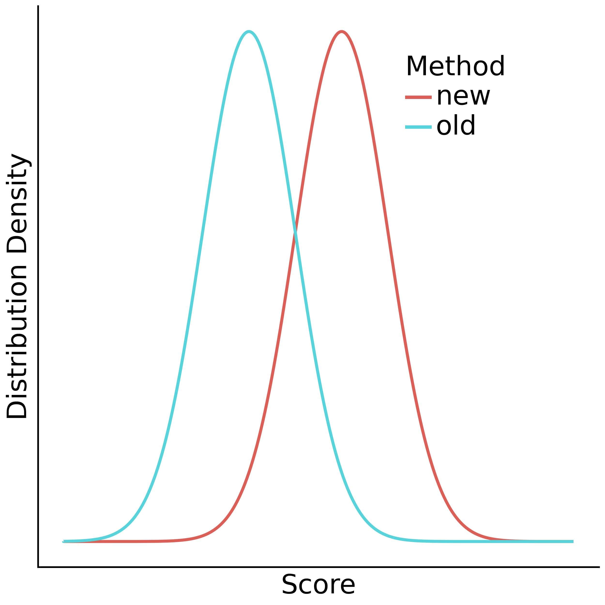
In this case, most values likely under the new method will be unlikely under the old one, and vice versa, because the distributions have the same shape. If they don’t, different means may have little to no practical significance. So, we always have to consider our implicit assumptions and formulate the effects so that they make sense.

4. Simple vs. Composite Null

Let $\theta$ be the parameter of interest. If the null specifies only one value $\boldsymbol{\theta_0}$ for $\boldsymbol{\theta}$ , we call it a simple null hypothesis. In that case, the alternative hypothesis is $H_a: \theta \neq \theta_0$ .

However, there are cases in which more than one value corresponds to the default or “no-effect” state. For example, we may be interested in knowing if the new teaching method is more efficient, not just if the new and old methods statistically differ. In that case, the effect we’re interested in finding out is $\mu_{old} < \mu_{new}$ . That’s our alternative hypothesis. The opposite, $\mu_{old} \geq \mu_{new}$ , corresponds to our null. It covers two ways in which the effect may not be there: the case in which two methods are equally efficient ( $\mu_{new} = \mu{old}$ ) and the case in which the old one works better ( $\mu_{old} > \mu_{new}$ ).

In general, if the null specifies multiple values for the tested parameter $\boldsymbol{\theta}$ , we call it a composite null hypothesis:

$[H_0: \theta \in \Theta_0]$

where $\Theta_0$ is the set of all the values for which, if $\theta$ took them, we say there is no effect.

In our example, $\theta = \mu_{old} - \mu_{new} \geq 0$ is the composite null, so ![\Theta_0 = 0, \infty).

4.1. The P-Value

Computing the -value for a composite null isn’t as straightforward as with a simple null. The reason is that the test statistic may follow different distributions under the values in $\Theta_0$ , so there isn’t one, but many distributions to consider when calculating the -value.

To resolve this, we can use the maximum $\boldsymbol{p}$ -value over all $\theta_0 \in \Theta_0$ :

$[\max_{\theta_0 \in \Theta_o} P(T \geq t^* \mid \theta = \theta_0)]$

assuming that higher values of the test statistic are less compatible with the null.

If we always use the maximum -value and reject the null if it’s lower than the threshold $\alpha$ , we can be sure that no matter the value of our parameter $\theta$ , the resulting error frequency will not be higher than $\alpha$ .

In the most common tests, such as the Student t test, the maximum -value usually corresponds to a boundary of $\Theta_0$ . In our teaching example, any difference $\mu_{old} - \mu_{new}$ greater than 0 yields lower -values.

5. Conclusion

In this article, we explained the null hypothesis in statistics. It corresponds to the no-effect state of the world. We reject it in favor of the alternative hypothesis if the observed effect is unlikely under the null.

Persistence

REST

Security