How to Invert PCA? | Baeldung中文网

1. Introduction

In real-world applications, we often deal with large datasets. In addition to millions of samples, we also work with high dimensions. To manage this complexity, we can reduce the dimensionality of our data by using Principal Component Analysis (PCA).

In this tutorial, we’ll show how to reverse the PCA and later discuss how discarding principal components (PC) affects data reconstruction.

Additionally, we point out another article for a complete treatise on PCA.

2. Overview of PCA and Its Inversion

Let’s briefly summarize how PCA works. Let the original dataset $X^{*} \in \mathbb{R}^{n \times p}$ have observations and variables.

First, we compute the mean for each of the columns of $X^{*}$ . This gives us $\mu = [\mu_1 \ldots \mu_p] \in \mathbb{R}^{1 \times p}$ which later will be useful to center the data. Now, we can compute PCA in five steps:

PCA steps

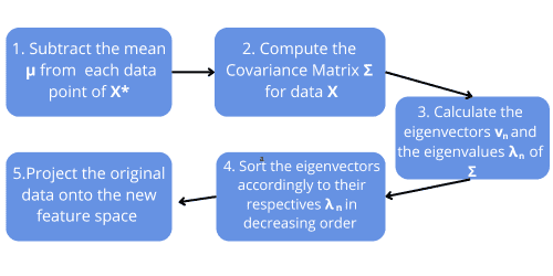
First, we center the data by repeating times each column of $\mu$ . To achieve that, we define $\mathbf{1}_n$ as a column vector of ones and compute:

$[X = X^{*} - \mathbf{1}_n\mu]$

Then, we compute the covariance matrix:

$[\Sigma = \frac{1}{n-1}X^{\top}X]$

In the third step, we calculate its eigenvectors and eigenvalues.

In the fourth step, we stack eigenvectors with the largest eigenvalues to build the matrix . This matrix has dimensions $p \times k$ . The eigenvectors define the new feature space. Typically, k < p .

Finally, we project the centered data onto the new feature space:

[Z=XW]

In the inversion task, we want to do the opposite: given the transformed data , our goal is to obtain the exact X^* or approximate X^* as closely as possible.

3. Reconstructing the Original Data

The formula to reconstruct the original data based on the PCA-transformed set is:

$[X_{rec} = ZW^{\top} + \mathbf{1}_n\mu]$

During the PCA, was obtained by projecting onto . So when we multiply by $W^{\top}$ , we’re projecting the data back to the original space.

This works because is orthogonal ( $WW^{\top}=\mathbf{I}$ ). The orthogonality ensures that we can reverse the projection by simply using the transposed of the eigenvector matrix.

We should also highlight that orthogonal transformations preserve the variance of the data.

We complete the inversion by adding the mean vector $\mu$ that was previously subtracted to center the data. That way, we restore the data to its original scale.

4. Information Loss

Reconstructed data suffer from information loss if we don’t preserve enough variance.

Let’s consider a four-dimensional dataset with five data points:

$[X^{*} = \begin{pmatrix} 1 & 0 & 0 & 0 \\ 0 & 1 & 0 & 0 \\ 0 & 0 & 1 & 0 \\ 0 & 0 & 0 & 1 \\ 1 & 1 & 1 & 1\end{pmatrix}]$

First, we compute the mean of each column:

$[\mu^{\top} = \begin{pmatrix} 0.4 \\ 0.4 \\ 0.4 \\ 0.4 \end{pmatrix}]$

We repeat five times the columns of $\mu$ and compute:

$[X = X^{*} - \mathbf{1}_5\mu = \begin{pmatrix} 1 & 0 & 0 & 0 \\ 0 & 1 & 0 & 0 \\ 0 & 0 & 1 & 0 \\ 0 & 0 & 0 & 1 \\ 1 & 1 & 1 & 1 \end{pmatrix} - \begin{pmatrix} 0.4 & 0.4 & 0.4 & 0.4 \\ 0.4 & 0.4 & 0.4 & 0.4 \\ 0.4 & 0.4 & 0.4 & 0.4 \\ 0.4 & 0.4 & 0.4 & 0.4 \\ 0.4 & 0.4 & 0.4 & 0.4 \end{pmatrix} = \begin{pmatrix} 0.6 & -0.4 & -0.4 & -0.4 \\ -0.4 & 0.6 & -0.4 & -0.4 \\ -0.4 & -0.4 & 0.6 & -0.4 \\ -0.4 & -0.4 & -0.4 & 0.6 \\ 0.6 & 0.6 & 0.6 & 0.6 \end{pmatrix} ]]$

Now, we compute the covariance matrix for the centered data:

$[\Sigma = \frac{1}{4} X^{\top}X =\begin{pmatrix} 1.2 & 0.2 & 0.2 & 0.2 \\ 0.2 & 1.2 & 0.2 & 0.2 \\ 0.2 & 0.2 & 1.2 & 0.2 \\ 0.2 & 0.2 & 0.2 & 1.2 \end{pmatrix}]$

Then, we compute and sort the eigenvalues:

$[\lambda_1 = 0.45, \quad \lambda_2 = 0.25, \quad \lambda_3 = 0.25, \quad \lambda_4 = 0.25]$

and the corresponding eigenvectors:

$[v_1 = \begin{pmatrix} 0.5 \\ 0.5 \\ 0.5 \\ 0.5 \end{pmatrix}, \quad v_2 = \begin{pmatrix} -0.16 \\ -0.59 \\ -0.03 \\ 0.79 \end{pmatrix}, \quad v_3 = \begin{pmatrix} -0.15 \\ 0.52 \\ -0.75 \\ 0.37 \end{pmatrix}, \quad v_4 = \begin{pmatrix} -0.87 \\ 0.29 \\ 0.29 \\ 0.29 \end{pmatrix}]$

To perform PCA on the data with the number of PCs k=3 , we define:

$[W = \begin{pmatrix} 0.5 & -0.16 & -0.15 \\ 0.5 & -0.59 & 0.52 \\ 0.5 & -0.03 & -0.75 \\ 0.5 & 0.79 & 0.37\end{pmatrix}]$

Now, we can compute :

$[Z = XW = \begin{pmatrix} -0.3 & -0.16 & -0.15\\ -0.3 & -0.59 & 0.52 \\ -0.3 & -0.03 & -0.75 \\ -0.3 & 0.79 & 0.37 \\ 1.2 & 0 & 0 \end{pmatrix}]$

4.1. Inverting PCA

We performed PCA on the data. Let’s now reverse it.

The reconstructed data of the inversion is given by:

$[X_{rec} = ZW^{\top} + \mu = \begin{pmatrix} 0.3 & 0.27 & 0.37 & 0.07 \\ 0.27 & 0.88 & -0.12 & -0.02 \\ 0.37 & -0.12 & 0.81 & -0.06 \\ 0.07 & -0.02 & -0.06 & 1.01 \\ 1 & 1 & 1 & 1\end{pmatrix}]$

We see that reducing the dimensionality from four to three resulted in a notable loss of information. The discrepancies between the original and reconstructed datasets indicate that the PCs didn’t capture enough variance of $X^{*}$ .

Numerically, the three PCs capture 0.38, 0.21, and 0.21 of the variance of the original dataset. So, the total explained variance of $X^{*}$ equals 0.8 , meaning we lost 20% of the original variance. That amount of lost information can be critical for some applications.

If we ran PCA with four PCs, the dimensionality would remain unchanged, and we could reconstruct the data precisely.

5. Approximation Error

We should also consider the approximation error of reconstruction.

Let’s consider the same dataset , but to simplify the notation, we denote the reconstructed data by $\hat{X}$ . In this section, we’ll present two different metrics to evaluate the approximation error. Let’s start with the traditional R-Square.

5.1. Root Mean Squared Error (RMSE)

Numerically, we can compute the Mean Squared Error (MSE) and the Root Mean Squared Error (RMSE):

$[\begin{aligned} \text{MSE} &= \frac{1}{n} \sum_{i=1}^{n} (x_i - \hat{x}_i)^2= 0.0045 \\ \text{RMSE} &= \sqrt{\frac{1}{n} \sum_{i=1}^{n} (x_i - \hat{x}_i)^2} = 0.212 \end{aligned}]$

5.2. Procrustes Disparity

Alternatively, we can use the Procrustes Disparity as a metric. This measure indicates how similar two matrices are after aligning them as closely as possible.

To compute this disparity, we start by centering both matrices and $\hat{X}$ by subtracting the respective means. Next, we scale them both to have a unit norm.

Finally, we apply the orthogonal transformation that minimizes the difference between the two matrices.

To define , we perform a SVD on $X^{\top}\hat{X}$ :

$[X^{\top}\hat{X} = U \Sigma V^{\top}]$

The transformation is given by:

$[R = VU^{\top}]$

We can compute the disparity as the Frobenius norm:

$[D = \| X^{\top} - \hat{X} R \|_F^2]$

In our example, we have D = 0.0259 .

6. Application to Image Denoising

Let’s see how PCA can reduce the noise in an image.

We start with a noiseless image and add a Gaussian noise with a variance equal to 0.015 .

The image is treated as a 2D matrix divided into patches. Our PCA is performed on a matrix of these patches that keep 90% of the variance in the noisy image. By doing so, we’re losing some of the variance, which is not a problem given that the noise also contributes to it.

Then, we reconstruct the denoised image and evaluate the result:

astronaut pca

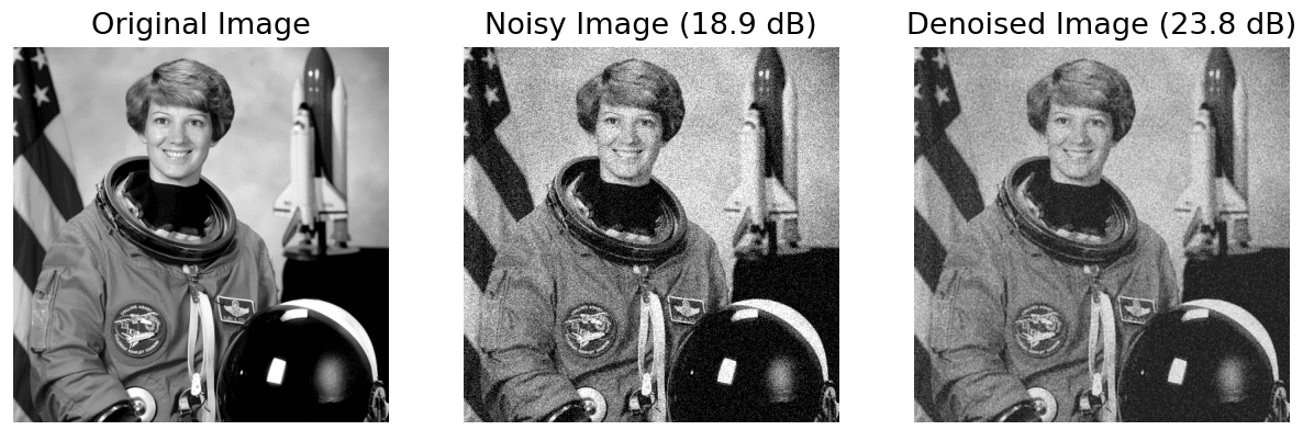
We choose SNR (Signal-to-Noise Ratio) as a metric given its robustness.

A higher SNR means a signal (in this case, the image) is stronger than noise. By discarding 10% of the variance in the noisy image, we can increase the SNR by almost 5 dB.

7. Conclusion

In this article, we briefly reviewed how to compute the PCA and presented how to reverse it and reconstruct the data.

Then, we saw that discarding principal components affected the quality of the reconstruction. We can evaluate the quality using different metrics.

Persistence

REST

Security