Eigenvectors and Eigenvalues | Baeldung中文网

1. Introduction

In this tutorial, we’ll study eigenvectors and eigenvalues.

2. Eigenvectors and Eigenvalues

We can define a vector as a geometric object with two properties: magnitude and direction. Generally speaking, most vectors change magnitude and direction when undergoing some linear transformation (described by a square matrix), such as rotation, stretch, or shear.

Eigenvectors are nonzero vectors that don’t change direction when a specific linear transformation occurs. Hence, an eigenvector of a transformation is only stretched when we apply that transformation. The corresponding eigenvalue is the scalar by which an eigenvector gets stretched or compressed. If it’s negative, the transformation reverses the direction of the eigenvector.

2.1. Intuition

An eigenvector is like a pivot on which the transformation matrix hinges within the scope of a specific operation. The eigenvalue tells us how vital this pivot is within the operation’s scope and relative to the eigenvalues of other eigenvectors.

An eigenvector is a skewer that helps us keep a set of linear transformations in place. The corresponding eigenvalue is the power of this skewer. The eigenvalue measures the distortion of the transformation, and the eigenvector signifies the orientation of the distortion.

3. Mathematical Analysis

3.1. Definition

Let be an $n\times n$ square matrix and be a nonzero column vector. Further on, we have a scalar $\lambda$ such that the following equation holds:

$[Ax = \lambda x]$

Then, $\lambda$ is an eigenvalue of , and is an eigenvector of corresponding to $\lambda$ . We call the set of all eigenvalues of a the spectrum of and denote it with $\sigma (A)$ .

3.2. Eigenvector Equation

Let’s delve deep into the above equation.

We can write this equation as $Ax = \lambda I x$ , where is the identity matrix of the same order $n \times n$ . Next, we rearrange all terms on the left :

$[Ax - \lambda I x = (A - \lambda I) x = O]$

Here, we use to denote the zero matrix. This homogenous equation system has variables and values. So, it will have a unique solution if and only if the determinants of both matrices are equal:

$[A - \lambda I = 0]$

To find the eigenvalues of any square matrix with dimensions $n \times n$ , we solve the characteristic equation $\det(A - \lambda I) = 0$ . That way, we get eigenvalues. Next, for each $\lambda$ , we find its corresponding eigenvector by substituting $\lambda$ in $(A - \lambda I) v = O$ and solving for using the elementary row transformations.

4. Example

We usually describe linear transformations in terms of matrices.

Let’s consider the following linear transformation matrix :

$[A = \left[ {\begin{array}{cc} 2 & 2 \\ 1 & 3 \\ \end{array} } \right]]$

To find its eigenvalues, we need $A - \lambda I$ :

$[A - \lambda I = \left[ {\begin{array}{cc} 2 & 2 \\ 1 & 3 \\ \end{array} } \right] - \lambda \left[ {\begin{array}{cc} 1 & 0 \\ 0 & 1 \\ \end{array} } \right] = \left[ {\begin{array}{cc} 2-\lambda & 2 \\ 1 & 3-\lambda \\ \end{array} } \right]]$

Now, we take the determinant:

$[\left|A - \lambda I\right| = \left|{\begin{array}{cc} 2 - \lambda & 2 \\ 1 & 3 - \lambda \\ \end{array} }\right| = \lambda^{2} - 5 \lambda + 4]$

Finally, we solve $\lambda^2 -5\lambda +4= 0$ for $\lambda$ :

$[\lambda^{2} - 5 \lambda + 4 = 0 \implies (\lambda - 1) (\lambda - 4) = 0]$

Thus, we get our two eigenvalues, $\lambda_{1}=1$ , and $\lambda_{2}=4$ .

4.1. Eigenvectors

Next, we use these eigenvalues to get our two eigenvectors $v_{1}$ and ${v_{2}$ . First, we find $v_{1}=[a b]^T$ for $\lambda_{1}=1$ :

$[(A - 1 I) v_{1} = \left[ {\begin{array}{cc} 1 & 2 \\ 1 & 2 \\ \end{array} }\right] \left[ {\begin{array}{c} a \\ b \\ \end{array} }\right]]$

Then, we use elementary row transformation to reduce the bottom row to o (subtract row 2 from row 1) and equate the result to the zero vector:

$[(A - I) v_{1} = \left[ {\begin{array}{cc} 1 & 2 \\ 0 & 0 \\ \end{array} }\right] \left[ {\begin{array}{c} a \\ b \\ \end{array} }\right] \implies a + 2b = 0]$

Since and can’t be zero, we get $a = -2b \in R \setminus \{0\}$ . This gives us our $v_{1}$ :

$[v_{1} = \left[ {\begin{array}{c} -2 \\ 1 \\ \end{array} }\right]]$

Similarly, we obtain our $v_{2}$ :

$[v_{2} = \left[ {\begin{array}{c} 1 \\ 1 \\ \end{array} }\right]]$

Also, any multiple of v_1 is the eigenvector of corresponding to the eigenvalue $\lambda_{1}=1$ , and the same holds for eigenvector $v_{2}$ .

4.2. Visualization

Let’s visualize what happens:

Eigen Plot - Visualization

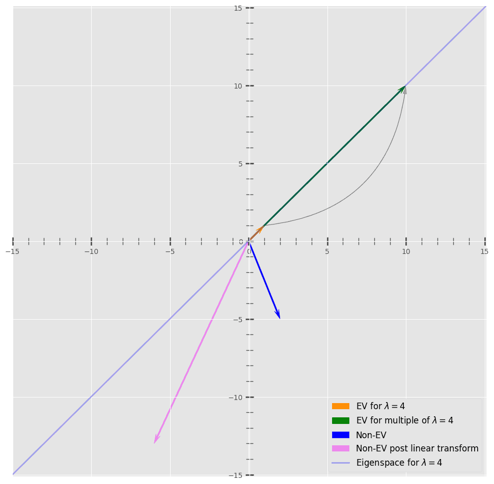
Here, we plotted $v_{2}$ and a non-eigenvector along with their transformations Av_2 and . Here, we can see that $v_{2}$ doesn’t change direction after applying , but does.

5. Applications

5.1. Dimensionality Reduction and Eigenvectors

We use eigenvectors and eigenvalues to reduce noise in our data (e.g., using principal component analysis (PCA)). This helps us improve the efficiency of our computationally intensive tasks.

Let’s say we are to open a wine shop. We have 100 different types of wine and only ten shelves to fit them all. We devise an allocation strategy to put similar wines on the same shelf. Each wine differs in taste, color, price, texture, origin, fizz, etc.

First, we must know which qualities are most important for grouping similar wines. We can solve this problem with principal component analysis (PCA). PCA gives us the principal component variables that explain the variation between different wine groups. Each principal component can be a single original feature or a combination of features.

To determine the principal components of the data, we calculate eigenvectors and eigenvalues from the covariance matrix (a matrix capturing correlation between data). Let’s say that 95% of the variability between wine sorts is explained by the first principal component (eigenvector with the most considerable absolute value of the corresponding eigenvalue).

In that case, we can organize wine bottles on our shelves. Each shelf will contain bottles of wines similar in value along his eigenvector’s axis.

6. Conclusion

In this article, we explained eigenvectors and eigenvalues. Eigenvalues and eigenvectors are associated with a square linear transformation matrix. An eigenvector is a nonzero vector that doesn’t change direction after applying a linear transformation. The corresponding eigenvalue is a scalar quantity that shows how much its magnitude changes.

Eigenvectors and eigenvalues are used in electrical circuits, mechanical systems, VLSI, deep learning, and graph algorithms (PageRank from Google). Moreover, all major computer vision tasks, such as face grouping, clustering, similarity search, dimensionality reductions, etc., use them in some form.

Persistence

REST

Security