布谷鸟哈希 | Baeldung中文网

1. Introduction

In this tutorial, we’ll study cuckoo hashing. We call it like this as its internal working closely mimics the behavior of a cuckoo.

Just as a newly hatched cuckoo baby kicks out other eggs or young ones from the nest, here, we kick out older keys from the hash table.

2. Hashing

Before starting, let’s briefly recap hashing!

In a hashing system, we store a key-value pair in each non-empty cell of a hash table. We mostly do it by applying a hash function to the data item’s key to get an integer we call a hash value. This points to a slot or an index in the hash table:

[hash = H(key)]

We use the hash function to find the location of a key in the hash table:

Generic Hashing

If the table has slots, H(k) needs to be lower than . We can achieve that by coupling with modulus division.

We retrieve our key-value pair by directly reading the slot from the table at the specified index we get using . This way, hashing offers us the benefit of inserting a value and reading it later in an amortized constant time ( $\boldsymbol{O(1)}$ ).

2.1. Collision in Hashing

Hashing works well with a large table, a small set of keys, and a hash function that maps values uniformly across the table. We don’t have collisions (two keys mapping to the same table index).

But collisions can happen in practice. We can solve this collision problem in two ways. In open hashing (or separate chaining), we store the keys that map to a given index in a link list. Further, we store the link list head in that table cell. Hence, on average, we insert an element in constant time ( $\boldsymbol{O(1)}$ ), but we take linear time to retrieve an element ( $\boldsymbol{O(k)}$ , where $k \approx n$ ).

In closed hashing or open addressing, we use additional buckets to store elements overflowing from their target bucket. Unlike open hashing, we don’t use any link list. Instead, we store all the keys in the hash table itself. Thus, our table size should be greater than the number of keys .

On average, we insert an element in constant time ( $\boldsymbol{O(1)}$ ), but we take linear time to retrieve an element ( $\boldsymbol{O(k)}$ , where $k \approx n$ ).

We employ different strategies for collision resolution. The easiest one is linear probing. However, we can also use cuckoo hashing.

3. Cuckoo Hashing

It was described by Rasmus Pagh and Flemming Friche Rodler in the year 2001. Cuckoo hashing is a type of closed hashing.

It uses two hash functions and two tables to avoid collisions. We pass our key to the first hash function to get a location in the first table. If that location is empty, we store the key and stop.

If it isn’t empty, we remove the old key stored there and store the current key in it. We then pass the old key to our second hash function to get a location in the second table. If we find that location empty, we store this old key there. Post that, we link the previous cell from table 1 and this cell from table 2.

If another key is already in that location in the second table, we remove it and store our old key from the first table. We also remove the link between the previous cell from table 1 and this cell from table 2.

We then pass this removed key k_2 from table 2 to our first hash function to get a location in the first table. If that location is empty, we store this key in that location. If it isn’t, we replace k_1 , the key previously stored in that location, with k_2 and remove the existing link.

After that, we link the previous cell from the second table to this cell of the first table and repeat this process with k_1 .

In case we get into a cycle, we have to rehash the entire table with new hash functions.

3.1. Formal Description

Let’s say our tables are $T_{1}$ , and $T_{2}$ . Each table is of size . Further, let hash functions be $h_{1}$ , and $h_{2}$ . Our key set is of size . Now, for a key , we pass it to $h_{1}$ to get its index in the first table. If the corresponding row is empty, then we store there.

Otherwise, there’ll be another key, which we denote with $k_{old}$ . We remove $k_{old}$ from the cell and store in it. This provides two possible locations in the hash table for each key. In one of the commonly used variants of the algorithm, the hash table is split into two smaller tables of equal size, and each hash function provides an index for one of these two tables.

3.2. Insertion

We now go through the pseudocode for insertion in cuckoo hashing:

algorithm Insert(k, table_1, table_2):
    // INPUT
    //    k = key to insert
    //    table_1 = first hash table
    //    table_2 = second hash table
    // OUTPUT
    //    Success if the insertion is successful, cycle rehash otherwise

    slot, table <- Search(k)
    if slot != empty and table != empty:
        // we already have the key k in table_1 or table_2
        return Success

    // Make a copy of input key
    k_current <- k
    i <- 1

    while k_current != k or i = 1:
        // hash k_current for table_1
        k1_old <- table_1[hash_1(k_current)]

        if k1_old = empty:
            // store k_current in the free slot in table_1
            table_1[hash_1(k_current)] <- k_current
            return Success
        else:
            // hash k1_old for table_2
            k2_old <- table_2[hash_2(k1_old)]
            if k2_old = empty:
                // store k1_old in that free slot in table_2
                table_2[hash_2(k1_old)] <- k1_old
                return Success
            else:
                k_current <- k2_old
        
        i <- i + 1

    // We encountered a cycle if we got here, so we rehash
    Rehash both tables and use different hash functions
    // Call Insert again
    return Insert(k)

3.3. Termination

There are two ways to stop: when we place all the keys successfully or run into a cycle (deadlock).

We’ll encounter a cycle when we end up with an unallocated key on the same table cell from where we started the replacement process. It happens when we run into a loop of hashing between the two tables and finally return to our starting point.

In that case, we need to use new hash functions to rehash all the keys stored in both tables. As a result, we can have multiple rounds of rehash operations before we finally place all our keys in the tables.

Alternatively, we can specify the maximal number of iterations allowed to spend trying to replace keys before resorting to rehashing. The rehashing operation works on all the keys stored in the tables and thus takes O(n) time.

4. Cuckoo Hashing Example

Let’s nail this concept with a working example.

4.1. Formal Setup

Let our key set be . Further, ={20, 33, 6, 45, 61, 11, 231, 90, 101, 122}. Let $h_{1}(x) = x\bmod11$ and $h_{2}(x) = x\bmod13$ . We’ll use two hash tables, $T_{1}$ (using $h_{1}$ ), and $T_{2}$ (using $h_{2}$ ). Both tables have 15 cells.

4.2. Workflow

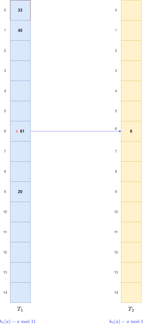
Let’s try to insert the first key, 20. We apply $h_{1}$ to 20 and store it in $slot_{9}$ of $T_{1}$ . Then, we store key 33 in $slot_{0}$ of $T_{1}$ . We follow the same process for the next two keys, 6 and 45: 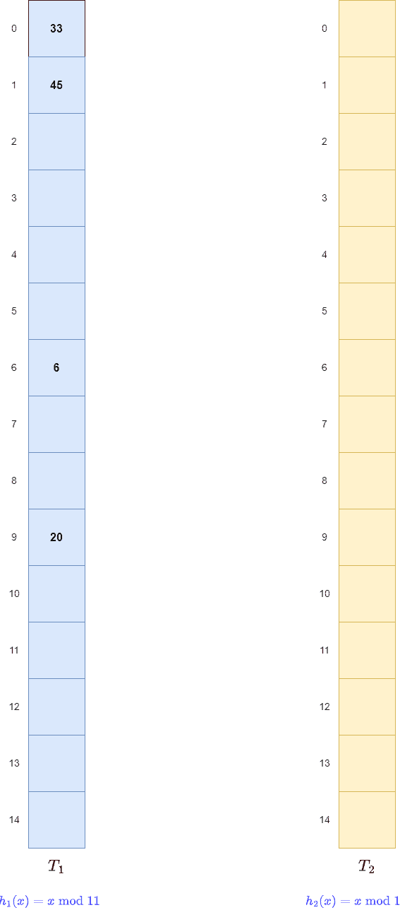Cuckoo Hashing 1 Next, key 61 maps t0 $slot_{6}$ of $T_{1}$ , but it is filled. So, like a cuckoo, we kick out the old key 6 and store key 61 there. Then, we apply $h_{2}$ to the old key 6. This gives us $slot_{6}$ of $T_{2}$ . 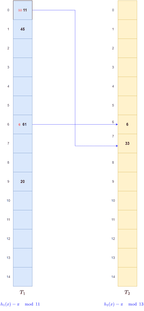As a result, we store it there and create a link between $slot_{60}$ of $T_{1}$ and $slot_{6}$ of $T_{2}$ : Cuckoo Hashing 2 Again, for key 11, we find $slot_{0}$ of $T_{1}$ filled with 33. So, we remove key 33 from there and store 11. Post that, we apply $h_{2}$ to 33 and store it in $slot_{7}$ of $T_{2}$ . We create a link between $slot_{0}$ of $T_{1}$ and $slot_{7}$ of $T_{2}$ : Cuckoo Hashing 3 We continue this way until we reach the last key, 122: 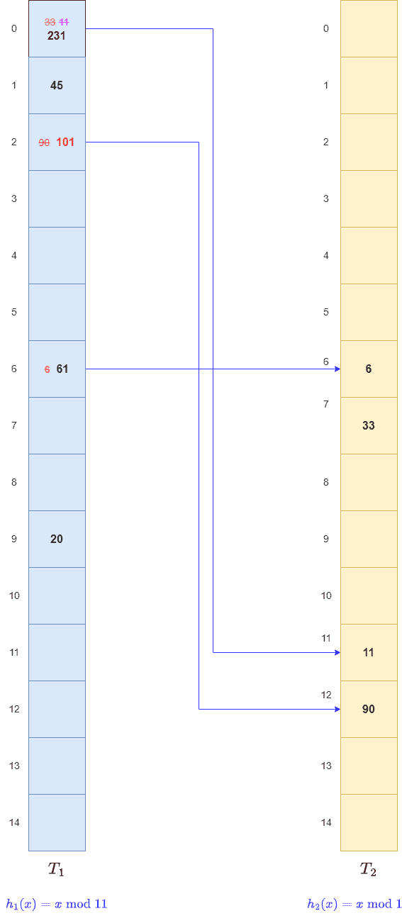Cuckoo Hashing 4 Here, we get $slot_{1}$ of $T_{1}$ , but this slot contains key 45. So, we remove 45 and store 122 there.

Next, we apply $h_{2}$ to key, 45 to get $slot_{6}$ of $T_{2}$ . However, we find it filled with key 6. So, we remove the key 6 and remove the old link from $slot_{6}$ of $T_{1}$ .

After that, we store key 45 there and create a link from $slot_{1}$ of $T_{1}$ to $slot_{6}$ of $T_{2}$ . Next, we apply $h_{1}$ on key 6 to get $slot_{6}$ of $T_{1}$ . But it already contains the key 61. So, we remove key 61 and store key 6 there.

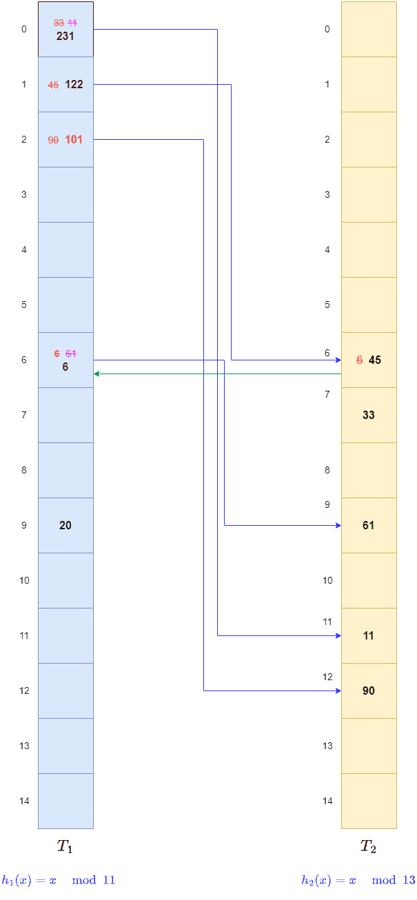We also create a link from $slot_{6}$ of $T_{2}$ to $slot_{6}$ of $T_{1}$ . Since h_1(61) points to slot_6 of T_1 , we apply $h_{2}$ to key 61 and store it on empty $slot_{9}$ of T_2 . We create a link from $slot_{6}$ of $T_{1}$ to $slot_{9}$ of $T_{2}$ : Cuckoo Hashing 5 This way, we hashed all the keys.

5. Hash Lookups

First, we apply our first hash function to the key. This gives us a slot in our first table. If the key is there, we stop. Otherwise, we apply our second hash function to the key and get a slot in the second table. If our key is hashed, it is there.

5.1. Example

Let’s use the same example from the above section. Let’s say we search for 33. So, h_1(33) gives us slot $slot_{0}$ of $T_{1}$ . But, we find key 231 there. So, we search our second table.

h_2(33) gives us slot $slot_{7}$ of $T_{2}$ . There, we find our key.

5.2. Pseudo Code

We now look at the pseudocode for the search operation:

algorithm Search(k):
    // INPUT
    //    k = the search key
    // OUTPUT
    //    the slot and table in which k is or should be

    tmp <- hash1(k)

    if table1[tmp] = k:
        // we found k in the first table table1
        slot <- tmp
        table <- table1
    else:
        // we try to find k in the second table table2
        slot <- hash2(k)
        table <- table2

    return slot, table

5.3. Time Complexity

The time complexity for the search operation is O(1) in cuckoo hashing. This is so because we perform at most two lookup operations for any key.

6. Conclusion

In this article, we studied the intricacies of hashing in general and cuckoo hashing in particular. Cuckoo hashing is a closed-form hashing where we eliminate collisions by using two hash functions and two tables.

Persistence

REST

Security