1. Introduction
In machine learning, feature selection is a crucial aspect that involves selecting only the most relevant and important features from a dataset.
This technique improves model performance, interpretability, and computational efficiency. In this article, we will explore various feature selection methods using the Python programming language.
We’ll discuss different approaches to feature selection and analyze their necessity, along with their benefits and shortcomings.
2. Why Do We Need Feature Selection?
In machine learning, datasets consist of objects described by features.
However, training models with too many features can introduce noise, slow the process, and lead to inaccurate predictions. Therefore, feature selection is essential to, extract useful data from the dataset and improve model accuracy by removing irrelevant features.
Feature selection methods enable businesses and organizations to extract meaningful insights from data, enhance decision-making processes, and develop more accurate and efficient machine-learning models tailored to specific domain requirements.
For example, the number of rooms and address are relevant features when predicting the sale price of a house, while the current owner’s name is not.
3. Feature Selection Methods
Feature selection methods aim to select the most relevant subset of features while dropping redundant, noisy, and irrelevant ones. There are several methods for feature selection:
3.1. Supervised & Unsupervised Methods
Unsupervised methods are applied to unlabeled data, and each feature is rated based on factors like entropy and variance.
On the other hand, supervised methods are applied to labeled data and maximize the supervised model’s performance.
3.2. Wrapper Methods
Wrapper methods evaluate feature subsets by training and evaluating the model iteratively. They use a greedy strategy to select features that maximize model performance.
Unlike filter methods, which rely solely on statistical measures, wrapper methods consider the performance of the model itself. One common wrapper method is Recursive Feature Elimination (RFE), which starts with all features, builds models with different feature subsets, and removes the least important features based on model performance.
3.3. Filter Methods
Filter methods use statistical tools to select feature subsets based on their relationship with the target variable. They remove features with low correlation with the target before training the final model.
Unlike wrapper methods, filter methods do not involve training the model iteratively. Instead, they evaluate each feature independently of the model. Common filter methods include techniques like variance thresholding, Chi-Square Test, Information Gain, and Pearson correlation.
3.4. Intrinsic Methods
Intrinsic methods perform feature selection implicitly during training. For example, decision trees select the best feature at each node split, representing feature selection.
Similarly, ensemble methods like Random Forests and Gradient Boosting Machines also implicitly perform feature selection by prioritizing the most informative features during the ensemble construction process.
3.5. Embedded Methods
Embedded methods, also known as integrated methods, perform feature selection as part of the model training process. These methods learn which features are most informative while simultaneously optimizing the model’s performance.
For instance, Lasso (L1 regularization) and Ridge (L2 regularization) regression are examples of embedded methods that penalize the coefficients of less important features.
4. Importing Libraries
The libraries that we’ll need in this article:
import numpy as np
import pandas as pd
import matplotlib.pyplot as plt

from sklearn.datasets import load_iris, load_wine

from sklearn.decomposition import PCA
from sklearn.feature_selection import VarianceThreshold, RFE
from sklearn.linear_model import LogisticRegression, LassoCV
from sklearn.ensemble import RandomForestClassifier
Scikit-learn, or sklearn, offers various algorithms for tasks like classification and regression. Supporting libraries include numpy and pandas for numerical computing and data manipulation, while matplotlib.pyplot aids in visualization. Specific modules like PCA and classifiers such as LogisticRegression highlight scikit-learn‘s versatility for preprocessing and modeling tasks.
5. Dataset Overview and Visualization
Before diving into feature selection techniques, let’s first explore the datasets we’ll be working with:
5.1. Iris Dataset (Supervised Learning)
The Iris dataset contains measurements of iris plant characteristics: sepal length, sepal width, petal length, and petal width. It consists of  samples, each belonging to one of three species: setosa, versicolor, or virginica.
Let’s visualize the first two features (sepal length and sepal width) to get an overview of the dataset.
# Load Iris dataset
iris_data = load_iris()
X_iris = iris_data.data
y_iris = iris_data.target

# Plot the first two features
plt.figure(figsize=(8, 6))
plt.scatter(X_iris[:, 0], X_iris[:, 1], c=y_iris, cmap='viridis', edgecolor='k')
plt.xlabel('Sepal Length (cm)')
plt.ylabel('Sepal Width (cm)')
plt.title('Iris Dataset: Sepal Length vs. Sepal Width')
plt.colorbar(label='Species')
plt.show()
The features of the Iris dataset are shown below: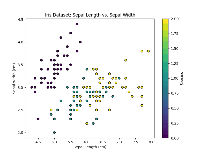
5.2. Wine Dataset (Unsupervised Learning)
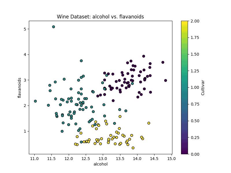
The Wine dataset contains the results of a chemical analysis of wines from three different cultivars. It consists of 178 samples and 13 features representing various chemical properties. Let’s visualize the first two features.
# Load Wine dataset
wine_data = load_wine()
X_wine = wine_data.data
y_wine = wine_data.target

# Select two features for visualization (e.g., Alcohol and Flavanoids)
feature1_index = 0  # Index of the first feature (Alcohol)
feature2_index = 6  # Index of the second feature (Flavanoids)

# Plot the selected features
plt.figure(figsize=(8, 6))
plt.scatter(X_wine[:, feature1_index], X_wine[:, feature2_index], c=y_wine, cmap='viridis', edgecolor='k')
plt.xlabel(wine_data.feature_names[feature1_index])
plt.ylabel(wine_data.feature_names[feature2_index])
plt.title('Wine Dataset: {} vs. {}'.format(wine_data.feature_names[feature1_index], wine_data.feature_names[feature2_index]))
plt.colorbar(label='Cultivar')
plt.show()
The first two features of the Wine dataset are alcohol and flavonoids:
6. Feature Selection Techniques
6.1. Variance Thresholding
Variance Thresholding is a filter methods technique. Features with low variance are often considered less informative. By setting a threshold, we can filter out features with variance below that threshold.
# Load Iris dataset
iris_data = load_iris()
X = iris_data.data

# Apply Variance Thresholding
selector = VarianceThreshold(threshold=0.2)
X_filtered = selector.fit_transform(X)

# Plot variances before and after filtering
plt.bar(range(X.shape[1]), np.var(X, axis=0), color='blue', label='Original')
plt.bar(range(X_filtered.shape[1]), np.var(X_filtered, axis=0), color='red', label='Filtered')
plt.xlabel('Feature Index')
plt.ylabel('Variance')
plt.title('Variance of Features before and after Filtering')
plt.legend()
# Save the plot
plt.savefig('Variance Threshold.png')
plt.show()
We can see the variance of features before and after filtering:
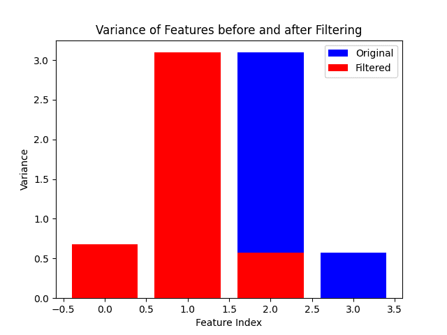
Variance thresholding helps identify features with low variability, which are less likely to contribute meaningfully to the model’s predictive power. The plot illustrates the effect of this technique in removing low-variance features, emphasizing its importance in feature selection.
6.2. Recursive Feature Elimination (RFE)
RFE is a wrapper method that recursively removes the least important features based on the coefficients of a machine learning model.
# Initialize RFE with Logistic Regression
lr = LogisticRegression()
rfe = RFE(lr, n_features_to_select=2)
rfe.fit(X, iris_data.target)

# Print selected feature names
selected_feature_names = np.array(iris_data.feature_names)[rfe.support_]
print("Selected Features:", selected_feature_names)
The output of the Python snippet:

RFE with Logistic Regression helps select the most relevant features for classification. By specifying the number of features to choose, we control the dimensionality of the final feature subset. This approach directly utilizes the coefficients of the logistic regression model, enhancing interpretability. In this case, features such as “petal length (cm)” and “petal width (cm)” are the most relevant.
6.3. L1 Regularization (Lasso)
Lasso regression penalizes the absolute size of the coefficients, leading to sparse solutions where irrelevant features have zero coefficients.
# Initialize LassoCV
lasso = LassoCV(cv=5)
lasso.fit(X, iris_data.target)

# Plot feature coefficients
plt.figure(figsize=(10, 5))
plt.bar(range(len(lasso.coef_)), lasso.coef_)
plt.xlabel('Feature Index')
plt.ylabel('Coefficient')
plt.title('Feature Coefficients with Lasso Regression')
# Save the plot
plt.savefig('Lasso Regression.png')
plt.show()
Lasso regression performs both feature selection and regularization: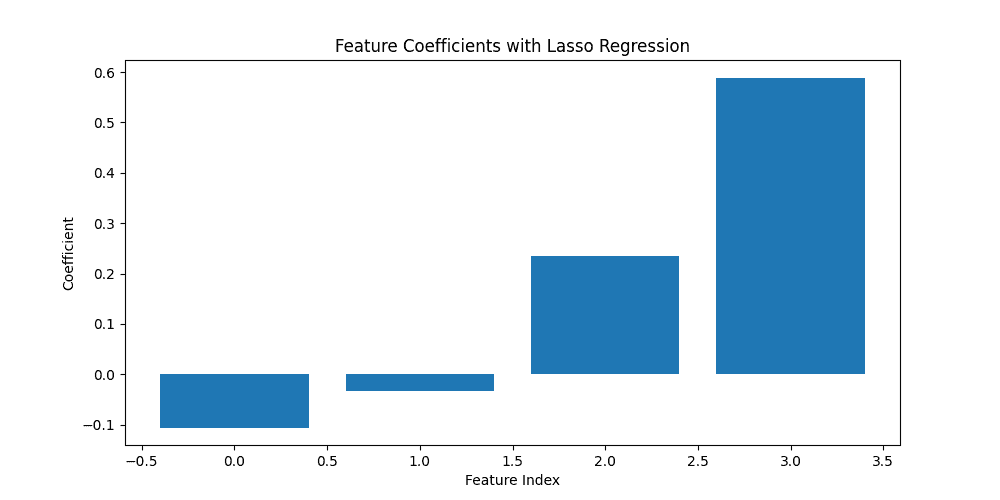
By visualizing the feature coefficients, we identify the most influential features in the model. Features with non-zero coefficients are considered important for prediction.
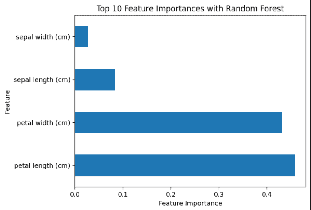
6.4. Random Forests
Random forests calculate feature importance based on how much the tree nodes that use a particular feature reduce impurity across all trees in the forest.
# Initialize Random Forest Classifier
rf = RandomForestClassifier()
rf.fit(X, iris_data.target)

# Plot feature importances
importances = pd.Series(rf.feature_importances_, index=iris_data.feature_names)
importances.nlargest(10).plot(kind='barh')
plt.xlabel('Feature Importance')
plt.ylabel('Feature')
plt.title('Top 10 Feature Importances with Random Forest')
# Save the plot
plt.savefig('Random Forest.png')
plt.show()
Random Forests offer a robust method for feature importance estimation. By visualizing the top features, we gain insights into which features have the most significant impact on model predictions:
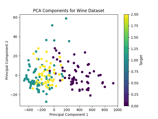
6.5. Principal Component Analysis (PCA)
For unsupervised learning, we’ll use the Wine dataset.
PCA is a dimensionality reduction technique that projects the data onto a lower-dimensional space while retaining most of its variance.
# Load Wine dataset
wine_data = load_wine()
X_wine = wine_data.data

# Apply PCA
pca = PCA(n_components=2)
X_pca = pca.fit_transform(X_wine)

# Plot PCA components
plt.scatter(X_pca[:, 0], X_pca[:, 1], c=wine_data.target, cmap='viridis')
plt.xlabel('Principal Component 1')
plt.ylabel('Principal Component 2')
plt.title('PCA Components for Wine Dataset')
plt.colorbar(label='Target')
# Save the plot
plt.savefig('PCA.png')
plt.show()
PCA reduces the dimensionality of the Wine dataset while preserving the variance as much as possible. By visualizing the data in the reduced space, we can observe the underlying structure and potential clusters:
7. Benefits and Challenges
Feature selection methods offer several benefits. First, they can reduce overfitting by removing redundant data and irrelevant features, such as outliers, that may affect the overall model performance. As a result, this method can improve accuracy. Moreover, by cleaning the data and dropping irrelevant characteristics of the dataset, we work with fewer columns, thus reducing training time.
However, we have to consider cases of high-dimensional data, in which there’s a risk of overfitting when there aren’t enough observations.
8. Real World Applications
Feature selection methods play a crucial role in various real-world applications across industries.
In finance, where predictive models are used for risk assessment and portfolio management, feature selection helps identify the most relevant financial indicators that impact asset performance or market trends.
Moreover, in healthcare, it aids in disease diagnosis and prognosis by identifying biomarkers or clinical features that are highly indicative of certain medical conditions.
Furthermore, in marketing and e-commerce, feature selection helps optimize advertising campaigns and recommendation systems by identifying customer behavior patterns and product preferences.
Also, in manufacturing and engineering, feature selection is utilized for predictive maintenance and quality control, where identifying key factors affecting product performance or equipment failure is essential for optimizing production processes and minimizing downtime.
9. Conclusion
Feature selection is fundamental in both supervised and unsupervised learning tasks, influencing model performance and interpretability.
In this article, we explored various techniques for feature selection in Python, covering both supervised and unsupervised learning scenarios. By applying these techniques to different datasets, we demonstrated their effectiveness and provided insights into their application and interpretation.