使用 Transformer 进行目标检测

1. Introduction

In this tutorial, we’ll learn about the DETR family of models for object detection in computer vision.

Meta AI first introduced DETR in the paper in 2020.

2. Object Detection

2.1. Definition

Object detection is a computer vision task in which we detect and locate objects of interest in an image or video.

The task involves two things. First, we need to identify the presence of an object of interest in the image. If we succeed, we estimate the position and boundaries of objects in an image.

Thus, the solution outputs a list of entries, with each entry consisting of the following fields:

1. Label (class of the object such as dog, cat)
2. Confidence score (estimated probability that the box contains an object described by the label)
3. Bounding box with its four coordinates (top left x, top left y, width, and height) of the box around the object)

2.2. Categorization

Based on the underlying detection approach, we can categorize object detection methods into two main types:

1. Single-stage methods
2. Double stage-methods

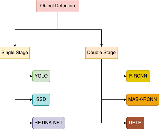
Single-stage methods, such as the YOLO or SSD family, scan through the image once during detection. So, they’re faster but with slightly low detection quality.

Conversely, double-stage methods pass through each image twice in the detection flow. This category prioritizes detection accuracy over speed. Models such as Faster R-CNN, Mask R-CNN, and Cascade R-CNN come under this category.

3. Object Detection Using DETR

The DETR model is an object detector based on transformers. It draws inspiration from the Mask R-CNN family of object detectors.

DETR combines the best of convolution (CNN), visual attention (transformers), and graphs (bipartite matching). It uses a well-established convolution backbone to extract a low-level feature map of the given image. Then, it feeds the feature map into a visual transformer architecture (encoder and decoder) to get a set of predictions. Lastly, it uses feedforward networks that work in parallel to directly predict the final set of detections by combining them with bipartite matching loss between predicted and ground-truth object detections.

Unlike YOLO, DETR doesn’t require prior constructs, such as spatial anchors (specific scales to detect objects at different stages in the architecture flow) or non-maximal suppression (to filter out duplicate boxes).

This model can be used for tasks such as bounding box detection, instance segmentation, keypoint detection, and dense pose detection. We can quickly obtain pre-trained models for each task to load and use on new images.

3.1. DETR Architecture

Let’s understand its architecture:

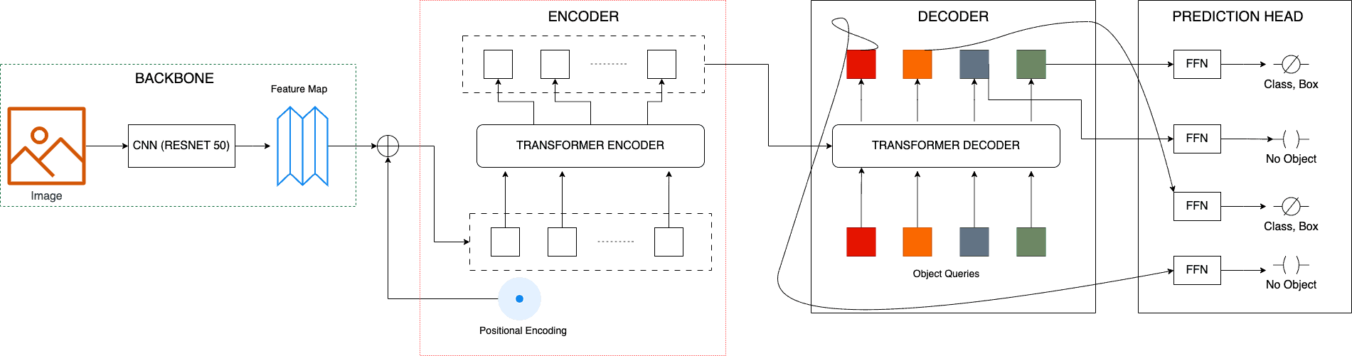
In DETR, we use a conventional CNN backbone (say Resnet 50) to learn a two-dimensional representation of an input image. We call it a feature map. Then, we flatten it (convert it from 2D to 1D) and chunkify it. After that, we add the positional encoding (sequential order since the transformer is position invariant). Finally, we use a transformer encoder to get a vector representation as an encoder output.

At the same time, we pass as input to the decoder a small preset number of learned positional embeddings (=100 by default) that we call object queries. The decoder takes these queries. Then, it derives keys and values from the encoder output. Now, it uses the attention mechanism for transformers.

Here, the model takes the scaled (by dimension of query vector) dot product of each query vector with all the key vectors in the image chunks. These scores indicate how much focus each encoded image chunk should receive for that query. We then pass the attention scores through a softmax function to get a probability distribution. After that, we weigh the value vectors with this probability. Finally, we take a weighted sum of the weighed value vector to create the new predictions.

We pass each output embedding of the decoder to shared feedforward networks (FFNs). Each FFN either outputs a , meaning it found no objects, or it predicts the class and bounding box for the found object.

3.2. Feedforward Networks

The last component of DETR consists of a series of FFNs.

Each FFN in DETR is a trilayer perceptron with a ReLU activation function, hidden dimension , and a linear projection layer.

The linear layer predicts the class label using a softmax function. It uses to represent that case of no object detection.

FFNs work parallel to predict the boxes’ normalized center coordinates, heights, and widths.

4. DETR Training Loss

Next, we move to the loss function.

DETR infers a fixed-size set of predictions in a single pass through the decoder. is a hyperparameter with a default value of 100.

The loss function function has two components:

1. Bipartite matching loss
2. Bounding box prediction loss

4.1. Bipartite Loss

For our ground truth , we denote our prediction set as . If there are fewer than objects, we pad with to make also a set of objects. A bipartite matching between these and is finding that permutation of elements that has the lowest cost:

   

Here, is a pair-wise matching cost between ground truth  and the prediction having index . We use the Hungarian algorithm to compute this assignment.

Now, each ground truth element is a tuple where denotes the target class label (including ) and is a four-dim vector that denotes ground truth box center coordinates and its height and width relative to the image size. For the prediction with index , let be the probability of predicting label and be the prediced box. With these notations, we define as:

   

Here is the box prediction loss that we describe next.

4.2. Box Prediction Loss

Next, we compute the box loss. We find that loss can have different scales for small and large boxes for the same relative errors. To minimize its impact, we use a linear combination of the and the generalized IoU (intersection over union) loss :

   

Here, and are hyperparameters. We normalize both losses by the number of objects inside our training batch.

4.3. Overall Loss

This is for one pair of ground truth and prediction. We can generalize it to cover all pairs to include negative log-likelihood for class prediction and a box loss :

   

Here,    is the optimal assignment computed in the section 4.1.

Thus, the DETR loss function has twin objectives. First, it attempts to optimize the bipartite matching between predicted and ground truth objects. Second, it minimizes overall loss by optimizing object-specific bounding box losses.

Since the overall loss function uniquely assigns a prediction to a ground truth object, it is invariant to a permutation of predicted objects. Thus, it can output all predictions in parallel.

5. Object Detection Using Pre-trained Model

Let’s look at an application using the detection model for object detection in Python using PyTorch. We can implement this in the TensorFlow framework.

5.1. Setup

First, we set up a virtual environment for this code. We can use the pyenv or virtualenv tools to create this environment. After activating the new environment, we should install all the necessary libraries:

1. torch
2. torchvision
3. pillow
4. transformers
5. numpy
6. requests
7. matplotlib

5.2. Libraries

Let’s load the necessary libraries:

import torch, torchvision
import torchvision.transforms as T
from PIL import Image
import requests, warnings
import matplotlib.pyplot as plt

warnings.filterwarnings("ignore")

5.3. Data

We’ll show the COCO dataset for this demo. COCO has the following 80 objects (11 objects are removed, so we write ‘N/A’):

CLASSES = [
    'N/A', 'person', 'bicycle', 'car', 'motorcycle', 'airplane', 'bus',
    'train', 'truck', 'boat', 'traffic light', 'fire hydrant', 'N/A',
    'stop sign', 'parking meter', 'bench', 'bird', 'cat', 'dog', 'horse',
    'sheep', 'cow', 'elephant', 'bear', 'zebra', 'giraffe', 'N/A', 'backpack',
    'umbrella', 'N/A', 'N/A', 'handbag', 'tie', 'suitcase', 'frisbee', 'skis',
    'snowboard', 'sports ball', 'kite', 'baseball bat', 'baseball glove',
    'skateboard', 'surfboard', 'tennis racket', 'bottle', 'N/A', 'wine glass',
    'cup', 'fork', 'knife', 'spoon', 'bowl', 'banana', 'apple', 'sandwich',
    'orange', 'broccoli', 'carrot', 'hot dog', 'pizza', 'donut', 'cake',
    'chair', 'couch', 'potted plant', 'bed', 'N/A', 'dining table', 'N/A',
    'N/A', 'toilet', 'N/A', 'tv', 'laptop', 'mouse', 'remote', 'keyboard',
    'cell phone', 'microwave', 'oven', 'toaster', 'sink', 'refrigerator', 'N/A',
    'book', 'clock', 'vase', 'scissors', 'teddy bear', 'hair drier',
    'toothbrush'
]

5.4. Model Inference

Let’s check out how to use the model:

model = torch.hub.load('facebookresearch/detr', 'detr_resnet50', pretrained=True)

model.eval();
url = 'http://images.cocodataset.org/train2017/000000000036.jpg'
im = Image.open(requests.get(url, stream=True).raw)

transform = T.Compose([
     T.Resize(800),
     T.ToTensor(),
     T.Normalize([0.485, 0.456, 0.406], [0.229, 0.224, 0.225])
])

img = transform(im).unsqueeze(0)

outputs = model(img)

We first load the pretrained DETR model and set it to inference mode. Then, we download an image from COCO and transform it to pass through the DETR model. Lastly, we pass the transformed image to the model to get predictions.

5.5. Visualization

Let’s plot the predictions at three confidence thresholds using the routines the Google Colab notebook:

conf = [0.9, 0.7, 0.0]
for threshold in conf:
    probas_to_keep, bboxes_scaled = filter_bboxes_from_outputs(outputs,
                                                            threshold=threshold)
plot_results(im, probas_to_keep, bboxes_scaled)

For the threshold of 0.9, our DETR detected a person and umbrella with a confidence of almost 100%:

For the confidence of 0.7, we see the same output:

For a threshold equal to 0, we see all of the 100 query slots:

Most query slots have a low confidence score, so we can set higher thresholds to filter out irrelevant queries.

6. DETR vs. CNNs

Let’s compare DETR with CNNs:

Property

CNN

DETR

Foundation

Convolution operation on image feature map followed by a fully connected classification layer.

Self-attention on an image chunk with all other chunks

Prior Constructs for detection

NMS, Anchors

Not required

Use of Graphs

Not explicitly used for detection

Bipartite graph matching

Accuracy

Low

High

Inference Time

Low

High

Receptive Bias

Low

High

Training Time

Low

Relatively higher

Design Complexity

Low

High

Model Size

Smaller

Slightly larger

Convolutional Neural Network (CNN) based systems directly predict object classification and localization in a single step. Hence, they are faster but need more points for accuracy.

On the other hand, DETR is a two-stage model that first uses CNN to extract features from an image. Then, it predicts regions with potential objects. It concludes by classifying and localizing those objects. Hence, we find it slower than single-stage detectors, but it scores more points regarding accuracy.

7. Conclusion

In this article, we learned about DETR for object detection.

DETR extracts image feature maps using a convolution backbone and then applies encoder and decoder transformers to derive detections using bipartite graph matching. It’s more accurate than a pure CNN model but has higher complexity, size, and turnaround time.